Deep Learning
Sanjiv R. Das
Professor of Finance and Data Science
Santa Clara University
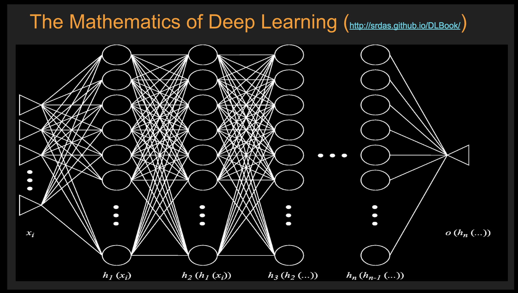
REFERENCE BOOK: http://srdas.github.io/DLBook
In [1]:
%pylab inline
import pandas as pd
from IPython.external import mathjax

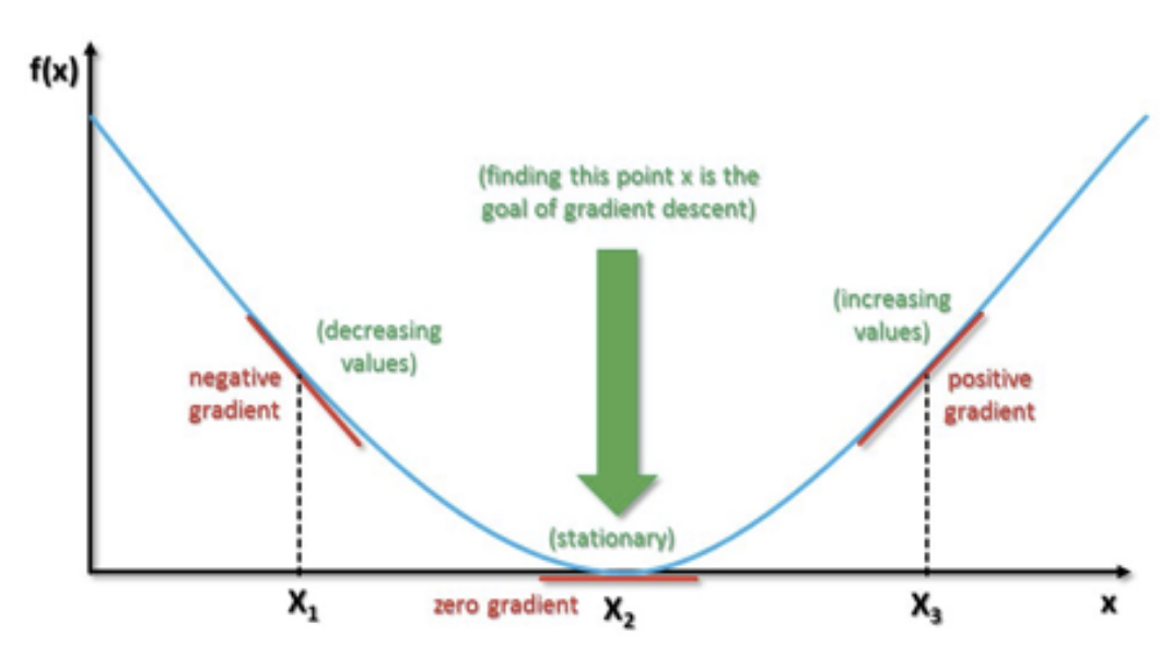
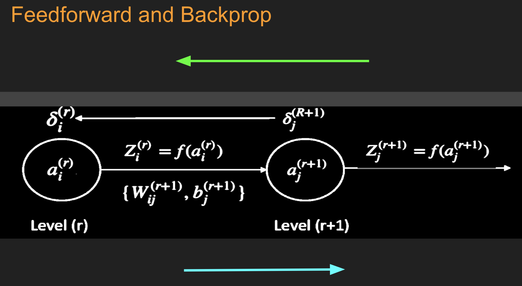
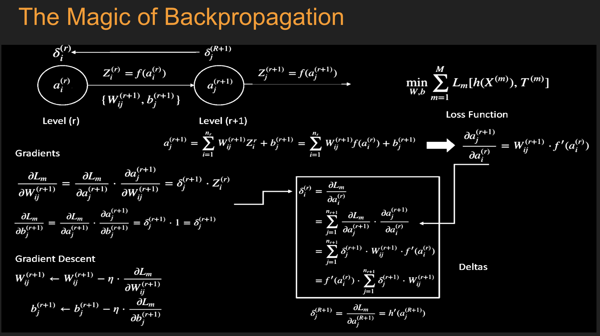
Batch Stochastic Gradient
Gradient Descent Example
In [2]:
def f(x):
    return 3*x**2 -5*x + 10

x = linspace(-4,4,100)
plot(x,f(x))
grid()

In [3]:
dx = 0.001
eta = 0.05  #learning rate
x = -3
for j in range(20):
    df_dx = (f(x+dx)-f(x))/dx
    x = x - eta*df_dx
    print(x,f(x))
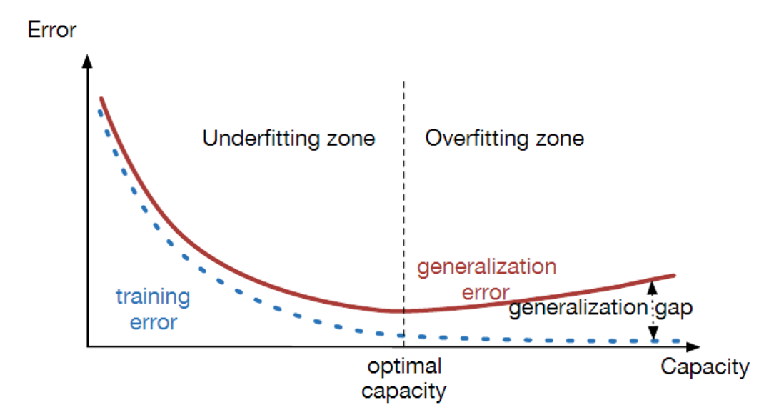
Under and Over-fitting
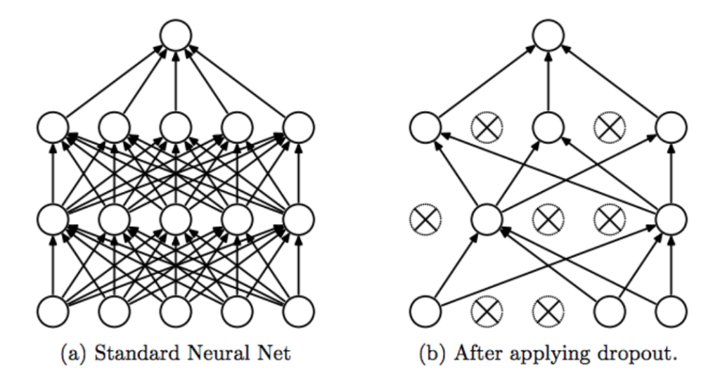
Dropout regularization

Pattern Recognition: Cancer
In [7]:
## Read in the data set
data = pd.read_csv("data/BreastCancer.csv")
data.head()
Out[7]:
In [9]:
## Convert the class variable into binary numeric
ynum = zeros((len(x),1))
for j in arange(len(y)):
    if y[j]=="malignant":
        ynum[j]=1
ynum[:10]
Out[9]:
In [10]:
## Make label data have 1-shape, 1=malignant
from keras import utils
y.labels = utils.to_categorical(ynum, num_classes=2)
#x = x.as_matrix()
print(y.labels[:10])
print(shape(x))
print(shape(y.labels))
print(shape(ynum))
In [11]:
## Define the neural net and compile it
from keras.models import Sequential
from keras.layers import Dense, Activation

model = Sequential()
model.add(Dense(32, activation='relu', input_dim=9))
model.add(Dense(32, activation='relu'))
model.add(Dense(32, activation='relu'))
model.add(Dense(1, activation='sigmoid'))
model.compile(optimizer='rmsprop',
              loss='binary_crossentropy',
              metrics=['accuracy'])
In [12]:
## Fit/train the model (x,y need to be matrices)
model.fit(x, ynum, epochs=25, batch_size=32,verbose=2)
Out[12]:
In [13]:
## Accuracy
yhat = model.predict_classes(x, batch_size=32)
acc = sum(yhat==ynum)
print("Accuracy = ",acc/len(ynum))

## Confusion matrix
from sklearn.metrics import confusion_matrix
confusion_matrix(yhat,ynum)
Out[13]:
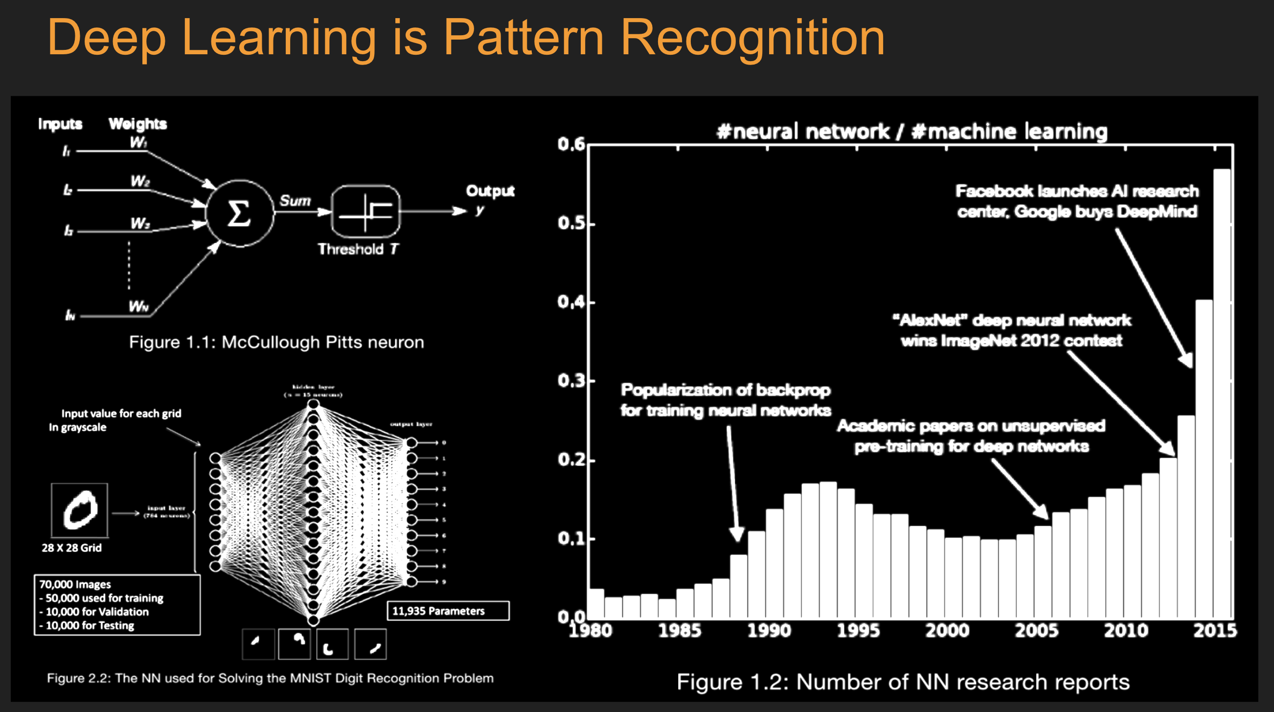
Another Canonical Example: Digit Recognition (MNIST)
- Extensible to many finance prediction problems.
- Information set: 784 (28 x 28) pixels for category prediction.
- Would you run a multinomial regression on these 784 columns.

In [14]:
## Read in the data set
train = pd.read_csv("data/train.csv", header=None)
test = pd.read_csv("data/test.csv", header=None)
print(shape(train))
print(shape(test))
In [15]:
## Reformat the data
X_train = train.as_matrix()[:,0:784]
Y_train = train.as_matrix()[:,784:785]
print(shape(X_train))
print(shape(Y_train))
X_test = test.as_matrix()[:,0:784]
Y_test = test.as_matrix()[:,784:785]
print(shape(X_test))
print(shape(Y_test))
y.labels = utils.to_categorical(Y_train, num_classes=10)
print(shape(y.labels))
print(y.labels[1:5,:])
print(Y_train[1:5])
In [16]:
hist(Y_train); grid()

In [17]:
## Define the neural net and compile it
from keras.models import Sequential
from keras.layers import Dense, Activation, Dropout
from keras.optimizers import SGD

data_dim = shape(X_train)[1]

model = Sequential([
    Dense(100, input_shape=(784,)),
    Activation('sigmoid'),
    Dense(100),
    Activation('sigmoid'),
    Dense(100),
    Activation('sigmoid'),
    Dense(100),
    Activation('sigmoid'),
    Dense(10),
    Activation('softmax'),
])

#model = Sequential()
#model.add(Dense(100, activation='sigmoid', input_dim=data_dim))
#model.add(Dropout(0.25))
#model.add(Dense(100, activation='sigmoid'))
#model.add(Dropout(0.25))
#model.add(Dense(100, activation='sigmoid'))
#model.add(Dropout(0.25))
#model.add(Dense(100, activation='sigmoid'))
#model.add(Dropout(0.25))
#model.add(Dense(10, activation='softmax'))
model.compile(optimizer='rmsprop',
              loss='categorical_crossentropy',
              metrics=['accuracy'])
In [18]:
## Fit/train the model (x,y need to be matrices)
model.fit(X_train, y.labels, epochs=10, batch_size=32,verbose=2)
Out[18]:
In [19]:
## In Sample
yhat = model.predict_classes(X_train, batch_size=32)

## Confusion matrix
from sklearn.metrics import confusion_matrix
cm = confusion_matrix(yhat,Y_train)
print(" ")
print(cm)

##
acc = sum(diag(cm))/len(Y_train)
print("Accuracy = ",acc)
In [20]:
## Out of Sample
yhat = model.predict_classes(X_test, batch_size=32)

## Confusion matrix
from sklearn.metrics import confusion_matrix
cm = confusion_matrix(yhat,Y_test)
print(" ")
print(cm)

##
acc = sum(diag(cm))/len(Y_test)
print("Accuracy = ",acc)
Learning the Black-Scholes Equation
See : Hutchinson, Lo, Poggio (1994)
In [23]:
from scipy.stats import norm
def BSM(S,K,T,sig,rf,dv,cp):  #cp = {+1.0 (calls), -1.0 (puts)}
    d1 = (math.log(S/K)+(rf-dv+0.5*sig**2)*T)/(sig*math.sqrt(T))
    d2 = d1 - sig*math.sqrt(T)
    return cp*S*math.exp(-dv*T)*norm.cdf(d1*cp) - cp*K*math.exp(-rf*T)*norm.cdf(d2*cp)

df = pd.read_csv('data/training.csv')
Normalizing spot and call prices
$C$ is homogeneous degree one, so $$ aC(S,K) = C(aS,aK) $$ This means we can normalize spot and call prices and remove a variable by dividing by $K$. $$ \frac{C(S,K)}{K} = C(S/K,1) $$
In [24]:
df['Stock Price'] = df['Stock Price']/df['Strike Price']
df['Call Price']  = df['Call Price'] /df['Strike Price']
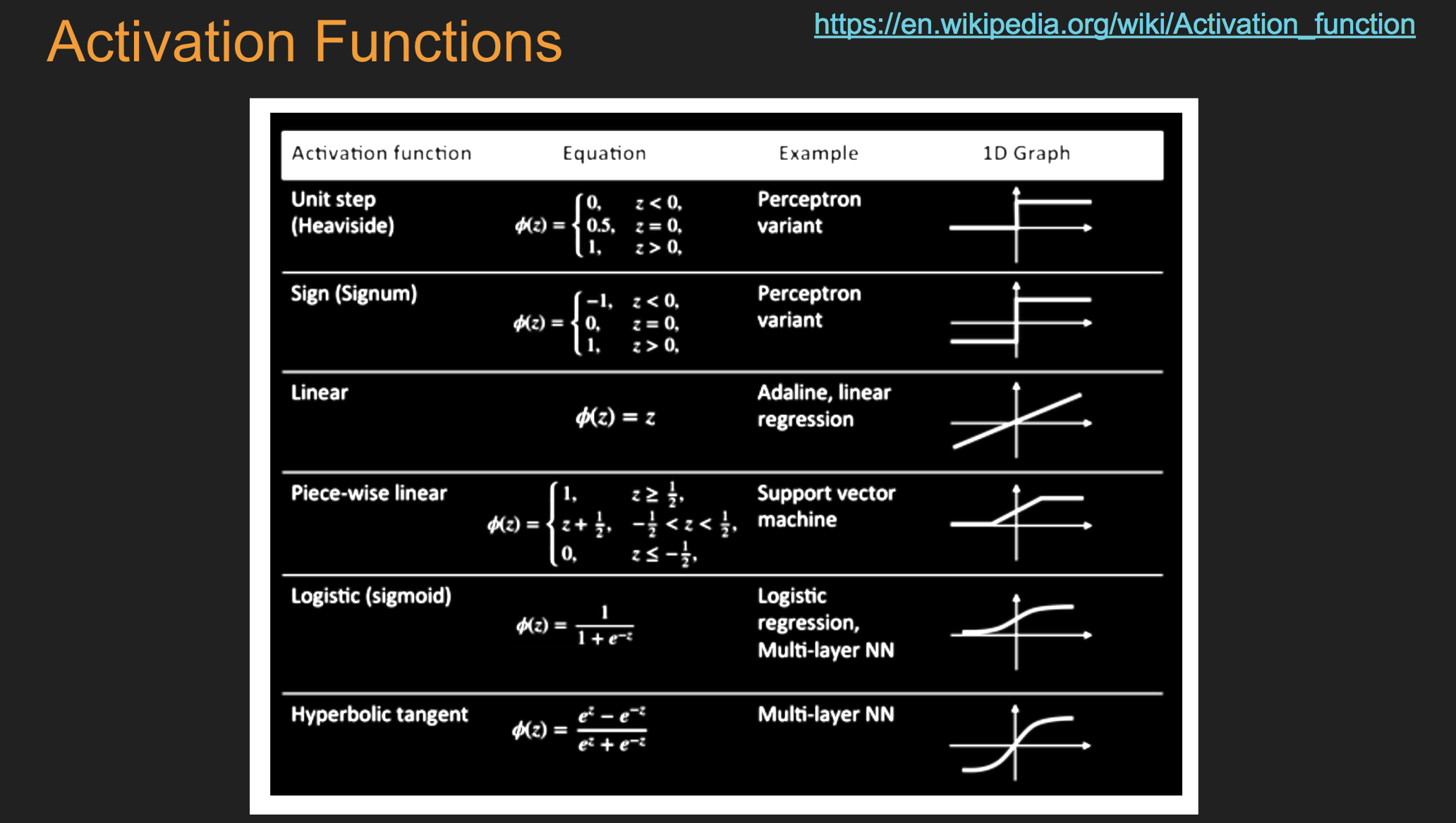
Data, libraries, activation functions
In [25]:
n = 300000
n_train =  (int)(0.8 * n)
train = df[0:n_train]
X_train = train[['Stock Price', 'Maturity', 'Dividends', 'Volatility', 'Risk-free']].values
y_train = train['Call Price'].values
test = df[n_train+1:n]
X_test = test[['Stock Price', 'Maturity', 'Dividends', 'Volatility', 'Risk-free']].values
y_test = test['Call Price'].values
In [26]:
#Import libraries
from keras.models import Sequential
from keras.layers import Dense, Dropout, Activation, LeakyReLU
from keras import backend

def custom_activation(x):
    return backend.exp(x)
Set up, compile and fit the model
In [27]:
nodes = 120
model = Sequential()

model.add(Dense(nodes, input_dim=X_train.shape[1]))
#model.add("relu")
model.add(Dropout(0.25))

model.add(Dense(nodes, activation='elu'))
model.add(Dropout(0.25))

model.add(Dense(nodes, activation='relu'))
model.add(Dropout(0.25))

model.add(Dense(nodes, activation='elu'))
model.add(Dropout(0.25))

model.add(Dense(1))
model.add(Activation(custom_activation))

model.compile(loss='mse',optimizer='rmsprop')

model.fit(X_train, y_train, batch_size=64, epochs=10, validation_split=0.1, verbose=2)
Out[27]:
Predict and check accuracy (in-sample)
In [36]:
y_train_hat = model.predict(X_train)
#reduce dim (240000,1) -> (240000,) to match y_train's dim
y_train_hat = squeeze(y_train_hat)
CheckAccuracy(y_train, y_train_hat)


Out[36]:
Predict and check accuracy (validation-sample)
In [37]:
y_test_hat = model.predict(X_test)
y_test_hat = squeeze(y_test_hat)
test_stats = CheckAccuracy(y_test, y_test_hat)


Random Forest of decision trees
A Random Forest uses several decision trees to make hypotheses about regions within subsamples of the data, then makes predictions based on the majority vote of these trees. This safeguards against overfitting/memorization of the training data.
Prepare Data
In [38]:
n = 300000
n_train =  (int)(0.8 * n)
train = df[0:n_train]
X_train = train[['Stock Price', 'Maturity', 'Dividends', 'Volatility', 'Risk-free']].values
y_train = train['Call Price'].values
test = df[n_train+1:n]
X_test = test[['Stock Price', 'Maturity', 'Dividends', 'Volatility', 'Risk-free']].values
y_test = test['Call Price'].values
Fit Random Forest
In [40]:
from sklearn.ensemble import RandomForestRegressor

forest = RandomForestRegressor()
forest = forest.fit(X_train, y_train)
y_test_hat = forest.predict(X_test)
In [41]:
stats = CheckAccuracy(y_test, y_test_hat)

