Logistic Regression

Sanjiv R. Das

In [16]:
%pylab inline
import pandas as pd
Populating the interactive namespace from numpy and matplotlib

Limited Dependent Variables

  • The dependent variable may be discrete, and could be binomial or multinomial. That is, the dependent variable is limited. In such cases, we need a different approach.

  • Discrete dependent variables are a special case of limited dependent variables. The Logit model we look at here is a discrete dependent variable model. Such models are also often called qualitative response (QR) models.

The Logistic Function

$$ y = \frac{1}{1+e^{-f(x_1,x_2,...,x_n)}} \in (0,1) $$

where

$$ f(x_1,x_2,...,x_n) = a_0 + a_1 x_1 + ... + a_n x_n \in (-\infty,+\infty) $$

In [20]:
#Sigmoid Function
def logit(fx):
    return exp(fx)/(1+exp(fx))

fx = linspace(-4,4,100)
y = logit(fx)
plot(fx,y)
xlabel('f(x)')
ylabel('Logit value')
grid()
In [3]:
#Import the SBA Loans dataset

sba = pd.read_csv("data/SBA.csv")
print(sba.columns)
Index(['LoanID', 'GrossApproval', 'SBAGuaranteedApproval', 'subpgmdesc',
       'ApprovalFiscalYear', 'InitialInterestRate', 'TermInMonths',
       'ProjectState', 'BusinessType', 'LoanStatus', 'RevolverStatus',
       'JobsSupported'],
      dtype='object')
In [4]:
#Feature engineering
sba["GuaranteePct"] = sba.SBAGuaranteedApproval.astype("float")/sba.GrossApproval.astype("float")
X = sba[['ApprovalFiscalYear', 'InitialInterestRate', 'TermInMonths',
        'RevolverStatus','JobsSupported','GuaranteePct']]
x1 = pd.get_dummies(sba.subpgmdesc)
#x1 = x1.drop(x1.columns[0],axis=1)
X = pd.concat([X,x1],axis=1)
x2 = pd.get_dummies(sba.BusinessType)
#x2 = x2.drop(x1.columns[0],axis=1)
X = pd.concat([X,x2],axis=1)
X.head()
Out[4]:
ApprovalFiscalYear InitialInterestRate TermInMonths RevolverStatus JobsSupported GuaranteePct 509 - DEALER FLOOR PLAN Community Advantage Initiative Community Express Contract Guaranty ... Patriot Express Revolving Line of Credit Exports - Sec. 7(a) (14) Rural Lender Advantage Seasonal Line of Credit Small Asset Based Small General Contractors - Sec. 7(a) (9) Standard Asset Based CORPORATION INDIVIDUAL PARTNERSHIP
0 2006 11.25 84 1 4 0.50 0 0 0 0 ... 0 0 0 0 0 0 0 1 0 0
1 2006 12.00 84 0 3 0.50 0 0 0 0 ... 0 0 0 0 0 0 0 1 0 0
2 2006 12.00 84 0 4 0.50 0 0 0 0 ... 0 0 0 0 0 0 0 0 1 0
3 2006 11.50 84 0 1 0.85 0 0 1 0 ... 0 0 0 0 0 0 0 1 0 0
4 2006 11.50 84 0 1 0.85 0 0 1 0 ... 0 0 0 0 0 0 0 1 0 0

5 rows × 26 columns

In [5]:
#Dependent categorical variable
y = pd.get_dummies(sba.LoanStatus)
y.head()
Out[5]:
CANCLD CHGOFF EXEMPT PIF
0 1 0 0 0
1 1 0 0 0
2 1 0 0 0
3 0 0 0 1
4 1 0 0 0
In [6]:
y.sum()
Out[6]:
CANCLD     58970
CHGOFF     66649
EXEMPT    245083
PIF       156998
dtype: int64
In [7]:
idx1 = list(where(y.CHGOFF==1)[0])
idx2 = list(where(y.PIF==1)[0])
idx = append(idx1,idx2)
print(len(idx))
X = X.iloc[idx]
X["Intercept"] = 1.0

y = y.CHGOFF.iloc[idx]
223647
In [8]:
from sklearn.linear_model import LogisticRegression
from sklearn.cross_validation import train_test_split
from sklearn import metrics
from sklearn.cross_validation import cross_val_score

# instantiate a logistic regression model, and fit with X and y
model = LogisticRegression()
model = model.fit(X, y)

# check the accuracy on the training set
model.score(X, y)
/Users/srdas/anaconda3/lib/python3.6/site-packages/sklearn/cross_validation.py:41: DeprecationWarning: This module was deprecated in version 0.18 in favor of the model_selection module into which all the refactored classes and functions are moved. Also note that the interface of the new CV iterators are different from that of this module. This module will be removed in 0.20.
  "This module will be removed in 0.20.", DeprecationWarning)
Out[8]:
0.8243750195620777
In [21]:
pd.DataFrame({'X':X.columns, 'Coeff':model.coef_[0]})
Out[21]:
X Coeff
0 ApprovalFiscalYear -0.000533
1 InitialInterestRate 0.348134
2 TermInMonths -0.041177
3 RevolverStatus -0.345469
4 JobsSupported -0.000225
5 GuaranteePct 0.268519
6 509 - DEALER FLOOR PLAN -0.004191
7 Community Advantage Initiative -0.000950
8 Community Express 0.467689
9 Contract Guaranty -0.022769
10 EXPORT IMPORT HARMONIZATION -0.002006
11 FA$TRK (Small Loan Express) -0.863875
12 Guaranty 0.609706
13 Gulf Opportunity -0.108411
14 International Trade - Sec, 7(a) (16) -0.000816
15 Lender Advantage Initiative -0.042409
16 Patriot Express 0.172032
17 Revolving Line of Credit Exports - Sec. 7(a) (14) -0.135843
18 Rural Lender Advantage -0.010936
19 Seasonal Line of Credit -0.003622
20 Small Asset Based -0.002782
21 Small General Contractors - Sec. 7(a) (9) -0.009936
22 Standard Asset Based -0.038550
23 CORPORATION 0.076209
24 INDIVIDUAL -0.034433
25 PARTNERSHIP -0.039321
26 Intercept 0.002332

Odds Ratio

What are odds ratios? An odds ratio (OR) is the ratio of probability of success to the probability of failure. If the probability of success is $p$, then

$$ OR = \frac{p}{1-p}; \quad \quad p = \frac{OR}{1+OR} $$

Odds Ratio Coefficients

  • In a linear regression, it is easy to see how the dependent variable changes when any right hand side variable changes. Not so with nonlinear models. A little bit of pencil pushing is required (add some calculus too).

  • The coefficient of an independent variable in a logit regression tell us by how much the log odds of the dependent variable change with a one unit change in the independent variable. If you want the odds ratio, then simply take the exponentiation of the log odds.

In [23]:
#Example

p = 0.3
OR = p/(1-p)
print('OR old =', OR)

beta = 2
OR_new = OR * exp(beta)
print('OR new =', OR_new)

p_new = OR_new/(1+OR_new)
print('p new =', p_new)
OR old = 0.4285714285714286
OR new = 3.1667383281131363
p new = 0.7600041276283266
In [10]:
# Evaluate the model by splitting into train and test sets
X_train, X_test, y_train, y_test = train_test_split(X, y, test_size=0.3, random_state=0)
model2 = LogisticRegression()
model2.fit(X_train, y_train)
Out[10]:
LogisticRegression(C=1.0, class_weight=None, dual=False, fit_intercept=True,
          intercept_scaling=1, max_iter=100, multi_class='ovr', n_jobs=1,
          penalty='l2', random_state=None, solver='liblinear', tol=0.0001,
          verbose=0, warm_start=False)
In [11]:
# Predict class labels for the test set
predicted = model2.predict(X_test)
print(predicted)
[0 0 0 ... 1 1 1]
In [12]:
# Generate class probabilities
probs = model2.predict_proba(X_test)
print(probs)
[[0.93284152 0.06715848]
 [0.95486653 0.04513347]
 [0.83622947 0.16377053]
 ...
 [0.30179065 0.69820935]
 [0.43927039 0.56072961]
 [0.23599253 0.76400747]]

Metrics

  1. Accuracy: the number of correctly predicted class values.

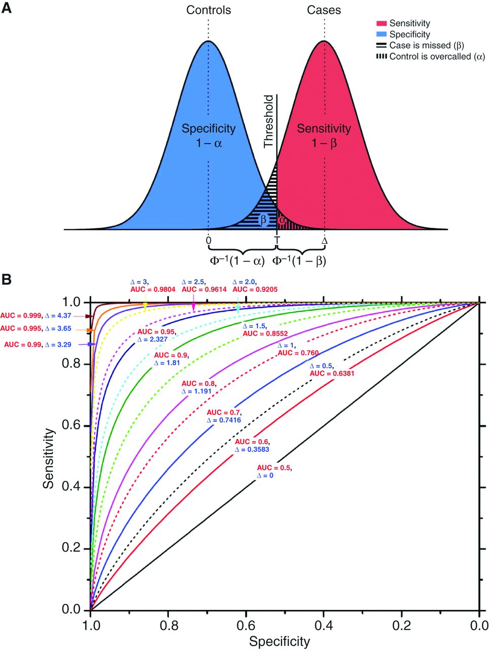
  2. ROC and AUC: The Receiver-Operating Characteristic (ROC) curve is a plot of the True Positive Rate (TPR) against the False Positive Rate (FPR) for different levels of the cut-off posterior probability. This is an essential trade-off in all classification systems.

  3. TPR = sensitivity or recall = TP/(TP+FN)

  4. FPR = (1 − specificity) = FP/(FP+TN)

AUC of the ROC curve

In [13]:
# generate evaluation metrics
print(metrics.accuracy_score(y_test, predicted))
print(metrics.roc_auc_score(y_test, probs[:, 1]))
0.827066100305537
0.8600518349121413

More Metrics

  1. Precision = $\frac{TP}{TP+FP}$

  2. Recall = $\frac{TP}{TP+FN}$

  3. F1 score = $\frac{2}{\frac{1}{Precision} + \frac{1}{Recall}}$

(F1 is the harmonic mean of precision and recall.)

In [15]:
print(metrics.confusion_matrix(y_test, predicted))
print(metrics.classification_report(y_test, predicted))
[[43753  3435]
 [ 8168 11739]]
             precision    recall  f1-score   support

          0       0.84      0.93      0.88     47188
          1       0.77      0.59      0.67     19907

avg / total       0.82      0.83      0.82     67095

Using R

  • We can also use the R programming language as it if often better suited to econometrics.

  • We will use a basketball data set this time for a change of pace.

  • The rpy2 package allows us to call R from a Python notebook. https://rpy2.bitbucket.io/

In [35]:
#Load R interface

%load_ext rpy2.ipython
In [27]:
%%R
#Read in the data
ncaa = read.table("data/ncaa.txt",header=TRUE)
print(dim(ncaa))
head(ncaa)
[1] 64 14
  No          NAME GMS  PTS  REB  AST   TO  A.T STL BLK   PF    FG    FT   X3P
1  1 NorthCarolina   6 84.2 41.5 17.8 12.8 1.39 6.7 3.8 16.7 0.514 0.664 0.417
2  2      Illinois   6 74.5 34.0 19.0 10.2 1.87 8.0 1.7 16.5 0.457 0.753 0.361
3  3    Louisville   5 77.4 35.4 13.6 11.0 1.24 5.4 4.2 16.6 0.479 0.702 0.376
4  4 MichiganState   5 80.8 37.8 13.0 12.6 1.03 8.4 2.4 19.8 0.445 0.783 0.329
5  5       Arizona   4 79.8 35.0 15.8 14.5 1.09 6.0 6.5 13.3 0.542 0.759 0.397
6  6      Kentucky   4 72.8 32.3 12.8 13.5 0.94 7.3 3.5 19.5 0.510 0.663 0.400
In [28]:
%%R
#Create the discrete dependent variable
y = c(rep(1,32),rep(0,32))
print(y)
 [1] 1 1 1 1 1 1 1 1 1 1 1 1 1 1 1 1 1 1 1 1 1 1 1 1 1 1 1 1 1 1 1 1 0 0 0 0 0 0
[39] 0 0 0 0 0 0 0 0 0 0 0 0 0 0 0 0 0 0 0 0 0 0 0 0 0 0
In [29]:
%%R
#FIT THE MODEL
x = as.matrix(ncaa[4:14])

h = glm(y~x, family=binomial(link="logit"))
names(h)
 [1] "coefficients"      "residuals"         "fitted.values"    
 [4] "effects"           "R"                 "rank"             
 [7] "qr"                "family"            "linear.predictors"
[10] "deviance"          "aic"               "null.deviance"    
[13] "iter"              "weights"           "prior.weights"    
[16] "df.residual"       "df.null"           "y"                
[19] "converged"         "boundary"          "model"            
[22] "call"              "formula"           "terms"            
[25] "data"              "offset"            "control"          
[28] "method"            "contrasts"         "xlevels"          
In [30]:
%%R
#RESULTS
summary(h)
Call:
glm(formula = y ~ x, family = binomial(link = "logit"))

Deviance Residuals: 
     Min        1Q    Median        3Q       Max  
-1.80174  -0.40502  -0.00238   0.37584   2.31767  

Coefficients:
             Estimate Std. Error z value Pr(>|z|)   
(Intercept) -45.83315   14.97564  -3.061  0.00221 **
xPTS         -0.06127    0.09549  -0.642  0.52108   
xREB          0.49037    0.18089   2.711  0.00671 **
xAST          0.16422    0.26804   0.613  0.54010   
xTO          -0.38405    0.23434  -1.639  0.10124   
xA.T          1.56351    3.17091   0.493  0.62196   
xSTL          0.78360    0.32605   2.403  0.01625 * 
xBLK          0.07867    0.23482   0.335  0.73761   
xPF           0.02602    0.13644   0.191  0.84874   
xFG          46.21374   17.33685   2.666  0.00768 **
xFT          10.72992    4.47729   2.397  0.01655 * 
xX3P          5.41985    5.77966   0.938  0.34838   
---
Signif. codes:  0 ‘***’ 0.001 ‘**’ 0.01 ‘*’ 0.05 ‘.’ 0.1 ‘ ’ 1

(Dispersion parameter for binomial family taken to be 1)

    Null deviance: 88.723  on 63  degrees of freedom
Residual deviance: 42.896  on 52  degrees of freedom
AIC: 66.896

Number of Fisher Scoring iterations: 6

Multinomial Logit

The probability of each class $(0,1,...,k)$ for $(k+1)$ classes is as follows:

$$ Pr[y=j] = \frac{e^{a_j^\top x}}{\sum_{i=1}^k e^{a_i^\top x}} $$

and

$$ Pr[y=0] = \frac{1}{\sum_{i=1}^k e^{a_i^\top x}} $$

Note that $\sum_{i=1}^k Pr[y=i] = 1$.

In [31]:
%%R
#CREATE 4 CLASSES THIS TIME
y = c(rep(3,16),rep(2,16),rep(1,16),rep(0,16))
print(y)
 [1] 3 3 3 3 3 3 3 3 3 3 3 3 3 3 3 3 2 2 2 2 2 2 2 2 2 2 2 2 2 2 2 2 1 1 1 1 1 1
[39] 1 1 1 1 1 1 1 1 1 1 0 0 0 0 0 0 0 0 0 0 0 0 0 0 0 0
In [37]:
%%R
#FIT THE MODEL

library(nnet)
res  = multinom(y~x)
# weights:  52 (36 variable)
initial  value 88.722839 
iter  10 value 71.549648
iter  20 value 61.992477
iter  30 value 51.299190
iter  40 value 45.868647
iter  50 value 44.083180
iter  60 value 43.077489
iter  70 value 42.899495
iter  80 value 42.810343
iter  90 value 42.801542
iter 100 value 42.784794
final  value 42.784794 
stopped after 100 iterations
In [38]:
%%R
#SHOW RESULTS
res
Call:
multinom(formula = y ~ x)

Coefficients:
  (Intercept)        xPTS       xREB       xAST        xTO       xA.T      xSTL
1    33.74486 0.422694013 -0.4806896 -0.9195585  0.7372724  2.7309094 0.1447635
2   -36.50899 0.004284913  0.5255269  0.4297660 -0.5497475 -0.6485187 0.6165437
3   -37.22782 0.122753359  0.2754536 -0.3991256 -0.1922775  3.6335713 1.5423808
       xBLK         xPF       xFG        xFT     xX3P
1 0.9647090 -0.70182622 -42.41196 -31.241416 4.455305
2 0.3488289  0.09580019  26.60137   1.879328 4.860927
3 0.3735845 -0.50986184  54.39210  -6.674520 9.199075

Residual Deviance: 85.56959 
AIC: 157.5696 
In [41]:
%%R
#SHOW FITTED PROBABILITIES
res$fitted.values
              0            1            2            3
1  1.888050e-05 4.133988e-06 2.230529e-01 7.769241e-01
2  1.330803e-03 3.190942e-06 3.117341e-01 6.869319e-01
3  4.268885e-03 1.216086e-02 1.715465e-01 8.120238e-01
4  4.159952e-03 3.936794e-04 3.803861e-01 6.150603e-01
5  4.305721e-05 6.180023e-04 9.099103e-03 9.902398e-01
6  2.540295e-03 2.361934e-03 3.400121e-02 9.610966e-01
7  4.378465e-01 3.763472e-02 1.064833e-01 4.180354e-01
8  1.560960e-02 6.345346e-03 1.836137e-01 7.944314e-01
9  1.080259e-01 6.295627e-01 8.084915e-02 1.815622e-01
10 1.053989e-02 1.460114e-01 1.061839e-02 8.328303e-01
11 1.464710e-02 7.228643e-05 6.150862e-02 9.237720e-01
12 4.417163e-02 2.863110e-01 4.492631e-01 2.202543e-01
13 5.998852e-01 1.363305e-01 1.525843e-01 1.112001e-01
14 1.575963e-03 3.291118e-04 1.450963e-01 8.529986e-01
15 8.447668e-02 7.769070e-02 1.751230e-01 6.627097e-01
16 2.092274e-04 1.265544e-05 7.310815e-03 9.924673e-01
17 3.414007e-01 1.609382e-01 4.661578e-01 3.150324e-02
18 6.360953e-02 3.932566e-02 4.464439e-01 4.506209e-01
19 5.664264e-01 9.403579e-02 3.338793e-01 5.658492e-03
20 1.104658e-01 3.566126e-04 3.312751e-01 5.579025e-01
21 1.064146e-03 1.568687e-03 8.832741e-01 1.140931e-01
22 3.652745e-01 6.335649e-05 6.170933e-01 1.756882e-02
23 1.066821e-03 4.314891e-04 3.808451e-01 6.176566e-01
24 4.532601e-04 1.321951e-04 8.115169e-01 1.878977e-01
25 2.130672e-02 3.078825e-04 7.939373e-01 1.844481e-01
26 8.125162e-01 1.330343e-01 4.082831e-02 1.362120e-02
27 3.406127e-01 1.077831e-01 4.243325e-01 1.272717e-01
28 5.252339e-03 3.193172e-02 6.693308e-01 2.934852e-01
29 3.276303e-01 8.959376e-06 6.511549e-01 2.120583e-02
30 3.277192e-02 8.947956e-02 8.513615e-01 2.638705e-02
31 1.776614e-02 3.096287e-03 8.735734e-01 1.055642e-01
32 6.193828e-02 4.927497e-02 7.095201e-01 1.792667e-01
33 4.771668e-02 2.537225e-01 2.888593e-02 6.696748e-01
34 1.003055e-01 7.434172e-01 2.579348e-02 1.304838e-01
35 4.765748e-03 9.947628e-01 9.556859e-05 3.758403e-04
36 1.398686e-04 9.083478e-01 9.849835e-03 8.166247e-02
37 4.073354e-01 5.323330e-01 6.029327e-02 3.830930e-05
38 3.294020e-01 6.206803e-01 3.352896e-02 1.638879e-02
39 6.052431e-07 9.999427e-01 7.888562e-08 5.661504e-05
40 3.798824e-01 5.392550e-01 4.267431e-03 7.659525e-02
41 1.804106e-01 5.931465e-01 2.079838e-01 1.845914e-02
42 3.706691e-01 6.282619e-01 9.818912e-04 8.710775e-05
43 5.156512e-02 7.515302e-01 3.338974e-04 1.965708e-01
44 1.201667e-04 9.998380e-01 2.272071e-06 3.957491e-05
45 3.539251e-03 9.858485e-01 4.199784e-03 6.412445e-03
46 1.543950e-01 4.760056e-01 7.809938e-02 2.915000e-01
47 8.627304e-01 1.358509e-01 1.339768e-03 7.894795e-05
48 2.335101e-02 6.031354e-01 2.549603e-01 1.185533e-01
49 5.705300e-01 1.441831e-03 4.141977e-01 1.383048e-02
50 4.774755e-01 7.674058e-03 4.143597e-01 1.004908e-01
51 7.528071e-01 8.713894e-02 1.403245e-01 1.972942e-02
52 5.928981e-01 2.726977e-01 1.260571e-01 8.347137e-03
53 5.144014e-01 2.353508e-03 4.702759e-01 1.296916e-02
54 7.325728e-02 5.593682e-02 7.444625e-01 1.263434e-01
55 9.831852e-01 1.484960e-02 1.963491e-03 1.706239e-06
56 6.108326e-01 2.966325e-01 8.430316e-02 8.231720e-03
57 4.904276e-01 7.764094e-03 4.963668e-01 5.441490e-03
58 7.380363e-01 8.871521e-04 2.482101e-01 1.286648e-02
59 1.173954e-02 9.837496e-01 6.030581e-04 3.907765e-03
60 4.266638e-01 4.181472e-01 7.204418e-02 8.314481e-02
61 4.667043e-01 3.002245e-01 4.465928e-04 2.326247e-01
62 2.453611e-01 7.546104e-01 2.815524e-05 2.966871e-07
63 9.965619e-01 8.909688e-06 3.281234e-03 1.479751e-04
64 7.104700e-01 1.302820e-05 2.894608e-01 5.614299e-05