Kaggle's Credit Card Fraud Dataset - RF
In this notebook I'll apply a Random Forest classifier to the problem, but first we will address the severe class imbalance of the set using the SMOTE ENN over/under-sampling technique.
Data is from: https://www.kaggle.com/dalpozz/creditcardfraud
%pylab inline
import pandas as pd
from sklearn.model_selection import train_test_split
from imblearn.combine import SMOTEENN
from sklearn.ensemble import RandomForestClassifier
from sklearn.metrics import accuracy_score
from sklearn.metrics import classification_report
from sklearn.metrics import roc_curve,auc
from sklearn.metrics import confusion_matrix
%%time
data = pd.read_csv('data/creditcard.csv')
print(data.shape)
print(data.head())
Quick Class counts
data[["Class","V1"]].groupby(["Class"]).count()
Mean Amount in Each class
data[["Class","Amount"]].groupby(["Class"]).mean()
X_train, X_test, y_train, y_test = train_test_split(data.drop('Class',axis=1), data['Class'], test_size=0.33)
print(X_train.shape)
print(y_train.shape)
print(X_test.shape)
print(y_test.shape)
Under/over-sample with SMOTE ENN to overcome class imbalance
While a Random Forest classifier is generally considered imbalance-agnostic, in this case the severity of the imbalance resuts in overfitting to the majority class.
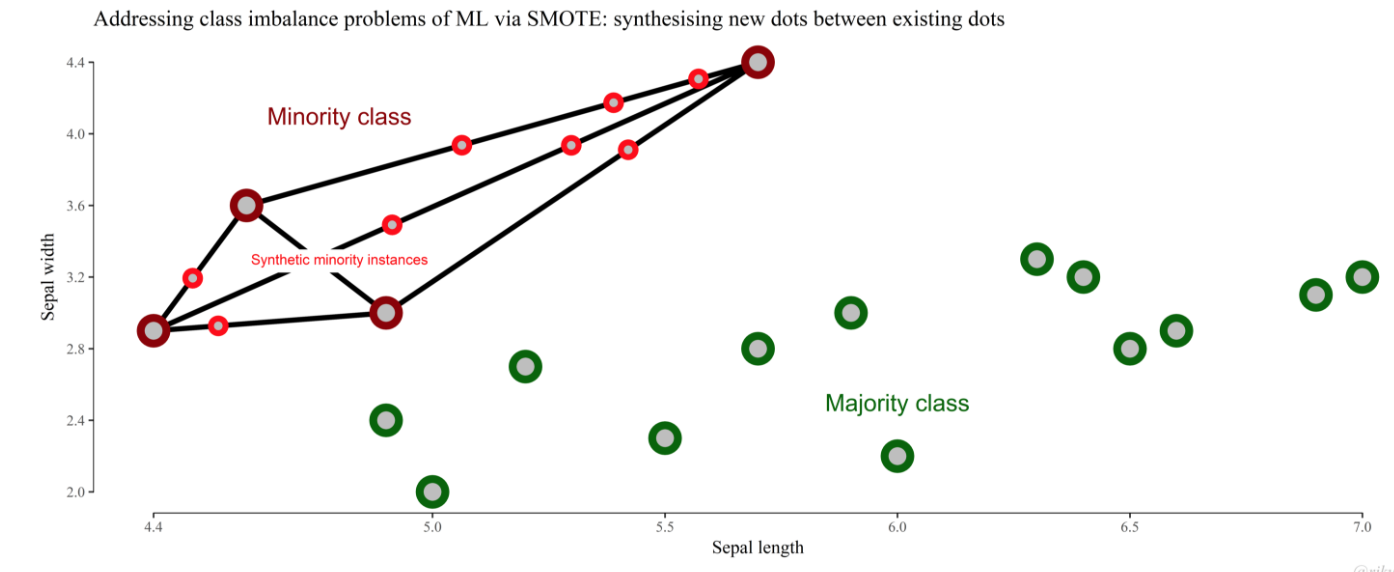
The Synthetic Minority Over-sampling Technique (SMOTE) is one of the most well-known methods to cope with it and to balance the different number of examples of each class.
The basic idea is to oversample the minority class, while trying to get the most variegated samples from the majority class.
Different types of Re-sampling methods: (see http://sci2s.ugr.es/noisebor-imbalanced)
- SMOTE in its basic version. The implementation of SMOTE used in this paper considers 5 nearest neighbors, the HVDM metric to compute the distance between examples and balances both classes to 50%.
- SMOTE + Tomek Links. This method uses tomek links (TL) to remove examples after applying SMOTE, which are considered being noisy or lying in the decision border. A tomek link is defined as a pair of examples $x$ and $y$ from different classes, that there exists no example $z$ such that $d(x,z)$ is lower than $d(x,y)$ or $d(y,z)$ is lower than $d(x,y)$, where $d$ is the distance metric.
- SMOTE-ENN. ENN tends to remove more examples than the TL does, so it is expected that it will provide a more in depth data cleaning. ENN is used to remove examples from both classes. Thus, any example that is misclassified by its three nearest neighbors is removed from the training set.
- SL-SMOTE. This method assigns each positive example its so called safe level before generating synthetic examples. The safe level of one example is defined as the number of positive instances among its k nearest neighbors. Each synthetic example is positioned closer to the example with the largest safe level so all synthetic examples are generated only in safe regions.
- Borderline-SMOTE. This method only oversamples or strengthens the borderline minority examples. First, it finds out the borderline minority examples P, defined as the examples of the minority class with more than half, but not all, of their m nearest neighbors belonging to the majority class. Finally, for each of those examples, we calculate its k nearest neighbors from P (for the algorithm version B1-SMOTE) or from all the training data, also with majority examples (for the algorithm version B2-SMOTE) and operate similarly to SMOTE. Then, synthetic examples are generated from them and added to the original training set.
## Keep original training data before SMOTE
X_train0 = X_train
y_train0 = y_train
sme = SMOTEENN()
X_train, y_train = sme.fit_sample(X_train, y_train)
print(X_train.shape)
print(y_train.shape)
unique(y_train, return_counts=True)
#SAVE TO PICKLE
import pickle
CCdata = {'X_train':X_train, 'X_test':X_test, 'y_train':y_train, 'y_test':y_test}
pickle.dump(CCdata, open( "data/CCdata.p", "wb" ))
mean(y_train) #Corresponds to counts from previous block
a = X_train[:,29]   #Collect the Amount column
print(mean(a))
print(mean(a[y_train==0]))
print(mean(a[y_train==1]))
Train & Predict
%%time
#DEFAULT: (~30 secs)
#class sklearn.ensemble.RandomForestClassifier(n_estimators=10,
#criterion=’gini’, max_depth=None, min_samples_split=2,
#min_samples_leaf=1, min_weight_fraction_leaf=0.0,
#max_features=’auto’, max_leaf_nodes=None, min_impurity_decrease=0.0,
#min_impurity_split=None, bootstrap=True, oob_score=False, n_jobs=1,
#random_state=None, verbose=0, warm_start=False, class_weight=None)[source]

clf = RandomForestClassifier(n_estimators=10)
clf = clf.fit(X_train,y_train)

y_test_hat = clf.predict(X_test)
Evaluate predictions
While the standard accuracy metric makes our predictions look near-perfect, we should bear in mind that the class imbalance of the set skews this metric.
Accuracy
#In sample
y_train_hat = clf.predict(X_train0)
accuracy_score(y_train0,y_train_hat)
#Out of sample
accuracy_score(y_test,y_test_hat)
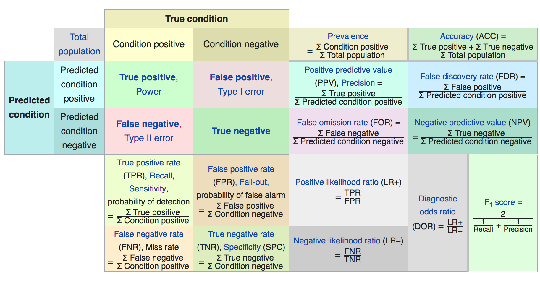
SciKitLearn's classification report gives us a more complete picture.
#print classification_report(y_test, y_test_hat)
print(classification_report(y_test, y_test_hat))
ROC Curve & AUC
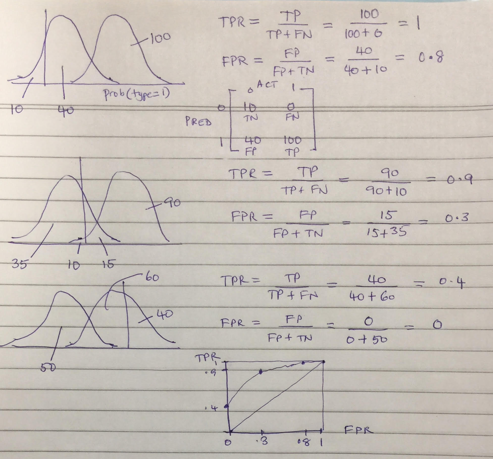
We'll plot the false positive rate (x-axis) against recall (true positive rate, y-axis) and compute the area under this curve for a better metric.
y_score = clf.predict_proba(X_test)[:,1]
fpr, tpr, _ = roc_curve(y_test, y_score)

title('Random Forest ROC curve: CC Fraud')
xlabel('FPR (Precision)')
ylabel('TPR (Recall)')

plot(fpr,tpr)
plot((0,1), ls='dashed',color='black')
plt.show()
#print 'Area under curve (AUC): ', auc(fpr,tpr)
print('Area under curve (AUC): ', auc(fpr,tpr))

Confusion Matrix
Another valuable way to visulize our predictions is to plot them in a confusion matrix, which shows us the frequency of correct & incorrect predictions.
def plot_confusion_matrix(cm, title='Confusion matrix', cmap=plt.cm.Blues):
    plt.imshow(cm, interpolation='nearest', cmap=cmap)
    plt.title(title)
    class_labels = ['Valid','Fraud']
    plt.colorbar()

    tick_marks = np.arange(len(class_labels))
    plt.xticks(tick_marks, class_labels, rotation=90)
    plt.yticks(tick_marks, class_labels)
    plt.tight_layout()
    plt.ylabel('True label')
    plt.xlabel('Predicted label')
cm = confusion_matrix(y_test, y_test_hat)
cm_normalized = cm.astype('float') / cm.sum(axis=1)[:, np.newaxis]
plt.figure(figsize=(5,5))
plot_confusion_matrix(cm_normalized, title='Normalized confusion matrix')

#Out of sample
print(cm)
print("False positive rate = ",cm[1][0]/sum(cm[1]))
#print classification_report(y_test, y_test_hat)
print(classification_report(y_test, y_test_hat))
#Type I error = 1 - precision
type1err = 1 - cm[1][1]/(cm[1][1]+cm[0][1])
print("Type I error =", type1err)
#Type II error = 1 - recall
type2err = 1 - cm[1][1]/(cm[1][1]+cm[1][0])
print("Type II error =", type2err)
#F1 score = harmonic mean of precision and recall
precision = cm[1][1]/(cm[1][1]+cm[0][1])
recall = cm[1][1]/(cm[1][1]+cm[1][0])
f_1 = 2.0/(1/precision + 1/recall)
print("F1 = ",f_1)
#Sensitivity = Recall = True positive rate = probability of detection
sensitivity = recall
print("Sensitivity = ",sensitivity)
#Specificity = true negative rate = TN/(TN+FP)
specificity = cm[0][0]/(cm[0][0]+cm[0][1])
print("Specificity = ",specificity)
#Recheck in sample
cm2 = confusion_matrix(y_train0, y_train_hat)
print(cm2)
print("False positive rate = ",cm2[1][0]/sum(cm[1]))
Logistic Regression
We now try the same classification with a Logit model, which is the baseline model we always try.
from sklearn.linear_model import LogisticRegression
logit = LogisticRegression()
logit.fit(X_train,y_train)
y_score = logit.predict_proba(X_test)[:,1]
fpr, tpr, _ = roc_curve(y_test, y_score)

title('Logit ROC curve: CC Fraud')
xlabel('FPR (Precision)')
ylabel('TPR (Recall)')

plot(fpr,tpr)
plot((0,1), ls='dashed',color='black')
plt.show()
#print 'Area under curve (AUC): ', auc(fpr,tpr)
print('Area under curve (AUC): ', auc(fpr,tpr))

y_test_hat = logit.predict(X_test)

cm = confusion_matrix(y_test, y_test_hat)
cm_normalized = cm.astype('float') / cm.sum(axis=1)[:, np.newaxis]
plt.figure(figsize=(5,5))
plot_confusion_matrix(cm_normalized, title='Normalized confusion matrix')

print(cm)
#print classification_report(y_test, y_test_hat)
print(classification_report(y_test, y_test_hat))
#Chisq test for significance of confusion matrix
from scipy.stats import chi2

cmA = cm
cmRowsums = matrix(cmA.sum(axis=1))
cmColsums = matrix(cmA.sum(axis=0))
cmE = cmRowsums.T.dot(cmColsums)/sum(cmA)
cmA = matrix(cm)
print("cmA = ",cmA)
print("cmE = ",cmE)

chisq_stat = sum((cmA-cmE)**2/cmE)
print("Chisq statistic = ",chisq_stat)
print("P-value = ",chi2.sf(chisq_stat,1))
ROC Curve Example