K Nearest Neighbors¶

Sanjiv R. Das¶

In [1]:

%pylab inline
import pandas as pd

Populating the interactive namespace from numpy and matplotlib

What is kNN?¶

This is one of the simplest algorithms for classification and grouping.
Simply define a distance metric over a set of observations, each with $M$ characteristics, i.e., $x_1,x_2,...,x_M$.

Compute the pairwise distance between each pair of observations, using any of the standard metrics. For example, Euclidian distance between data $x$ and $y$:

$$ d = \sqrt{\sum_{i=1}^M (x_i - y_i)^2} $$

Next, fix $k$, the number of nearest neighbors in the population to be considered.
Finally, assign the category based on which one has the majority of nearest neighbors to the case we are trying to classify.

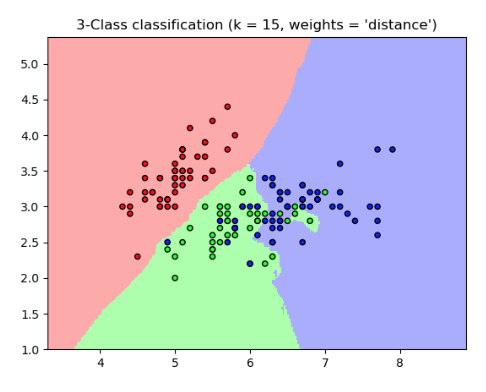
Classified Neighborhoods¶

In [2]:

#PREDICTION ON TEST DATA
from sklearn.metrics import accuracy_score
from sklearn.metrics import classification_report
from sklearn.metrics import roc_curve,auc
from sklearn.metrics import confusion_matrix

NCAA Dataset¶

In [3]:

ncaa = pd.read_table("data/ncaa.txt")
yy = append(list(ones(32)), list(zeros(32)))
ncaa["y"] = yy
ncaa.head()

Out[3]:

	No NAME	GMS	PTS	REB	AST	TO	A/T	STL	BLK	PF	FG	FT	3P	y
0	1. NorthCarolina	6	84.2	41.5	17.8	12.8	1.39	6.7	3.8	16.7	0.514	0.664	0.417	1.0
1	2. Illinois	6	74.5	34.0	19.0	10.2	1.87	8.0	1.7	16.5	0.457	0.753	0.361	1.0
2	3. Louisville	5	77.4	35.4	13.6	11.0	1.24	5.4	4.2	16.6	0.479	0.702	0.376	1.0
3	4. MichiganState	5	80.8	37.8	13.0	12.6	1.03	8.4	2.4	19.8	0.445	0.783	0.329	1.0
4	5. Arizona	4	79.8	35.0	15.8	14.5	1.09	6.0	6.5	13.3	0.542	0.759	0.397	1.0

In [4]:

#CREATE FEATURES
y = ncaa['y']
X = ncaa.iloc[:,2:13]
X.head()

Out[4]:

	PTS	REB	AST	TO	A/T	STL	BLK	PF	FG	FT	3P
0	84.2	41.5	17.8	12.8	1.39	6.7	3.8	16.7	0.514	0.664	0.417
1	74.5	34.0	19.0	10.2	1.87	8.0	1.7	16.5	0.457	0.753	0.361
2	77.4	35.4	13.6	11.0	1.24	5.4	4.2	16.6	0.479	0.702	0.376
3	80.8	37.8	13.0	12.6	1.03	8.4	2.4	19.8	0.445	0.783	0.329
4	79.8	35.0	15.8	14.5	1.09	6.0	6.5	13.3	0.542	0.759	0.397

In [36]:

#FIT MODEL
from sklearn.neighbors import NearestNeighbors as KNN
model = KNN(n_neighbors=5, algorithm='ball_tree')
model.fit(X)
distances, indices = model.kneighbors(X)
print(indices[:6])

[[ 0 23  3  4 22]
 [ 1 15 10  2 32]
 [ 2 26  4 27  3]
 [ 3  2  0 26 27]
 [ 4  2 38  3  0]
 [ 5 16 45 32 10]]

In [24]:

nn_sum = [sum(y[j]) for j in indices]
ypred = [1 if j>2 else 0 for j in nn_sum]
print(ypred)

[1, 1, 1, 1, 1, 1, 0, 1, 0, 0, 1, 1, 0, 1, 1, 1, 1, 1, 1, 1, 1, 1, 1, 1, 1, 1, 1, 1, 1, 1, 1, 1, 1, 1, 0, 0, 1, 0, 0, 0, 0, 0, 0, 0, 0, 1, 0, 0, 1, 0, 0, 0, 0, 1, 0, 0, 1, 0, 0, 0, 0, 0, 0, 0]

In [25]:

#CONFUSION MATRIX
cm = confusion_matrix(y, ypred)
cm

Out[25]:

array([[25,  7],
       [ 4, 28]])

In [26]:

#ACCURACY
accuracy_score(y,ypred)

Out[26]:

0.828125

In [29]:

#CLASSIFICATION REPORT
print(classification_report(y, ypred))

             precision    recall  f1-score   support

        0.0       0.86      0.78      0.82        32
        1.0       0.80      0.88      0.84        32

avg / total       0.83      0.83      0.83        64

Credit Card Dataset¶

In [31]:

#LOAD IN CREDIT CARD DATA
import pickle
CCdata = pickle.load(open("data/CCdata.p", "rb"))
X_train = CCdata['X_train']
y_train = CCdata['y_train']
X_test = CCdata['X_test']
y_test = CCdata['y_test']

In [43]:

#FIT MODEL
from sklearn.neighbors import KNeighborsClassifier as KNNC
model = KNNC(n_neighbors=5, algorithm='ball_tree')
model.fit(X_train, y_train)

Out[43]:

KNeighborsClassifier(algorithm='ball_tree', leaf_size=30, metric='minkowski',
           metric_params=None, n_jobs=1, n_neighbors=5, p=2,
           weights='uniform')

In [44]:

#CONFUSION MATRIX
ypred = model.predict(X_test)
cm = confusion_matrix(y_test, ypred)
cm

Out[44]:

array([[86086,  7741],
       [   74,    86]])

In [45]:

#ACCURACY
accuracy_score(y_test,ypred)

Out[45]:

0.9168502026876058

In [46]:

#CLASSIFICATION REPORT
print(classification_report(y_test, ypred))

             precision    recall  f1-score   support

          0       1.00      0.92      0.96     93827
          1       0.01      0.54      0.02       160

avg / total       1.00      0.92      0.95     93987

In [47]:

#ROC, AUC
y_score = model.predict_proba(X_test)[:,1]
fpr, tpr, _ = roc_curve(y_test, y_score)

title('ROC curve')
xlabel('FPR (Precision)')
ylabel('TPR (Recall)')

plot(fpr,tpr)
plot((0,1), ls='dashed',color='black')
plt.show()
print('Area under curve (AUC): ', auc(fpr,tpr))

Area under curve (AUC):  0.7396254542935403