Discriminant Analysis¶

Sanjiv R. Das¶

In [1]:

%pylab inline
import pandas as pd

Populating the interactive namespace from numpy and matplotlib

Credit Card Dataset¶

In [2]:

#LOAD IN CREDIT CARD DATA
import pickle
CCdata = pickle.load(open("data/CCdata.p", "rb"))
X_train = CCdata['X_train']
y_train = CCdata['y_train']
X_test = CCdata['X_test']
y_test = CCdata['y_test']

In [3]:

hist(y_train,3)
show()

In [4]:

hist(y_test,3)
show()

Linear Discriminant Analysis¶

http://srdas.github.io/MLBook/DiscriminantFactorAnalysis.html#discriminant-analysis

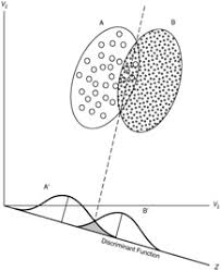
Discriminant Function¶

$$ D = a_1 x_1 + a_2 x_2 + ... + a_K x_K = \sum_{k=1}^K a_k x_k $$

$D$ is often replace by $Z$, which leads to the notion of "Z-score" or discriminant score.

In [5]:

#FIT THE LDA MODEL 
from sklearn.discriminant_analysis import LinearDiscriminantAnalysis as LDA
model = LDA()
model.fit(X_train, y_train)

Out[5]:

LinearDiscriminantAnalysis(n_components=None, priors=None, shrinkage=None,
              solver='svd', store_covariance=False, tol=0.0001)

In [6]:

#PREDICTION ON TEST DATA
from sklearn.metrics import accuracy_score
from sklearn.metrics import classification_report
from sklearn.metrics import roc_curve,auc
from sklearn.metrics import confusion_matrix

y_hat = model.predict(X_test)

In [7]:

#ACCURACY
#Out of sample
accuracy_score(y_test,y_hat)

Out[7]:

0.98610446125528

In [8]:

#CLASSIFICATION REPORT
print(classification_report(y_test, y_hat))

             precision    recall  f1-score   support

          0       1.00      0.99      0.99     93827
          1       0.09      0.83      0.17       160

avg / total       1.00      0.99      0.99     93987

In [9]:

#ROC, AUC
y_score = model.predict_proba(X_test)[:,1]
fpr, tpr, _ = roc_curve(y_test, y_score)

title('ROC curve')
xlabel('FPR (Precision)')
ylabel('TPR (Recall)')

plot(fpr,tpr)
plot((0,1), ls='dashed',color='black')
plt.show()
print('Area under curve (AUC): ', auc(fpr,tpr))

Area under curve (AUC):  0.973067187483347

In [10]:

#CONFUSION MATRIX
cm = confusion_matrix(y_test, y_hat)
cm

Out[10]:

array([[92548,  1279],
       [   27,   133]])

NCAA Dataset¶

In [11]:

ncaa = pd.read_table("data/ncaa.txt")
yy = append(list(ones(32)), list(zeros(32)))
ncaa["y"] = yy
ncaa.head()

Out[11]:

	No NAME	GMS	PTS	REB	AST	TO	A/T	STL	BLK	PF	FG	FT	3P	y
0	1. NorthCarolina	6	84.2	41.5	17.8	12.8	1.39	6.7	3.8	16.7	0.514	0.664	0.417	1.0
1	2. Illinois	6	74.5	34.0	19.0	10.2	1.87	8.0	1.7	16.5	0.457	0.753	0.361	1.0
2	3. Louisville	5	77.4	35.4	13.6	11.0	1.24	5.4	4.2	16.6	0.479	0.702	0.376	1.0
3	4. MichiganState	5	80.8	37.8	13.0	12.6	1.03	8.4	2.4	19.8	0.445	0.783	0.329	1.0
4	5. Arizona	4	79.8	35.0	15.8	14.5	1.09	6.0	6.5	13.3	0.542	0.759	0.397	1.0

In [12]:

#CREATE FEATURES
y = ncaa['y']
X = ncaa.iloc[:,2:13]
X.head()

Out[12]:

	PTS	REB	AST	TO	A/T	STL	BLK	PF	FG	FT	3P
0	84.2	41.5	17.8	12.8	1.39	6.7	3.8	16.7	0.514	0.664	0.417
1	74.5	34.0	19.0	10.2	1.87	8.0	1.7	16.5	0.457	0.753	0.361
2	77.4	35.4	13.6	11.0	1.24	5.4	4.2	16.6	0.479	0.702	0.376
3	80.8	37.8	13.0	12.6	1.03	8.4	2.4	19.8	0.445	0.783	0.329
4	79.8	35.0	15.8	14.5	1.09	6.0	6.5	13.3	0.542	0.759	0.397

In [13]:

#FIT MODEL
model = LDA()
model.fit(X,y)
ypred = model.predict(X)

In [14]:

#CONFUSION MATRIX
cm = confusion_matrix(y, ypred)
cm

Out[14]:

array([[27,  5],
       [ 5, 27]])

In [15]:

#ACCURACY
accuracy_score(y,ypred)

Out[15]:

0.84375

In [16]:

#CLASSIFICATION REPORT
print(classification_report(y, ypred))

             precision    recall  f1-score   support

        0.0       0.84      0.84      0.84        32
        1.0       0.84      0.84      0.84        32

avg / total       0.84      0.84      0.84        64

In [17]:

#ROC, AUC
y_score = model.predict_proba(X)[:,1]
fpr, tpr, _ = roc_curve(y, y_score)

title('ROC curve')
xlabel('FPR (Precision)')
ylabel('TPR (Recall)')

plot(fpr,tpr)
plot((0,1), ls='dashed',color='black')
plt.show()
print('Area under curve (AUC): ', auc(fpr,tpr))

Area under curve (AUC):  0.92578125