Chapter 10 Extracting Dimensions: Discriminant and Factor Analysis
10.1 Introduction
In discriminant analysis (DA), we develop statistical models that differentiate two or more population types, such as immigrants vs natives, males vs females, etc. In factor analysis (FA), we attempt to collapse an enormous amount of data about the population into a few common explanatory variables. DA is an attempt to explain categorical data, and FA is an attempt to reduce the dimensionality of the data that we use to explain both categorical or continuous data. They are distinct techniques, related in that they both exploit the techniques of linear algebra.
10.2 Discriminant Analysis
In DA, what we are trying to explain is very often a dichotomous split of our observations. For example, if we are trying to understand what determines a good versus a bad creditor. We call the good vs bad the “criterion” variable, or the “dependent” variable. The variables we use to explain the split between the criterion variables are called “predictor” or “explanatory” variables. We may think of the criterion variables as left-hand side variables or dependent variables in the lingo of regression analysis. Likewise, the explanatory variables are the right-hand side ones.
What distinguishes DA is that the left-hand side (lhs) variables are essentially qualitative in nature. They have some underlying numerical value, but are in essence qualitative. For example, when universities go through the admission process, they may have a cut off score for admission. This cut off score discriminates the students that they want to admit and the ones that they wish to reject. DA is a very useful tool for determining this cut off score.
In short, DA is the means by which quantitative explanatory variables are used to explain qualitative criterion variables. The number of qualitative categories need not be restricted to just two. DA encompasses a larger number of categories too.
10.3 Notation and assumptions
- Assume that there are \(N\) categories or groups indexed by \(i=2...N\).
- Within each group there are observations \(y_j\), indexed by \(j=1...M_i\). The size of each group need not be the same, i.e., it is possible that \(M_i \neq M_j\).
- There are a set of predictor variables \(x = [x_1,x_2,\ldots,x_K]'\). Clearly, there must be good reasons for choosing these so as to explain the groups in which the \(y_j\) reside. Hence the value of the \(k\)th variable for group \(i\), observation \(j\), is denoted as \(x_{ijk}\).
- Observations are mutually exclusive, i.e., each object can only belong to any one of the groups.
- The \(K \times K\) covariance matrix of explanatory variables is assumed to be the same for all groups, i.e., \(Cov(x_i) = Cov(x_j)\). This is the homoskedasticity assumption, and makes the criterion for choosing one class over the other a simple projection on the \(z\) axis where it may be compared to a cut off.
10.4 Discriminant Function
DA involves finding a discriminant function \(D\) that best classifies the observations into the chosen groups. The function may be nonlinear, but the most common approach is to use linear DA. The function takes the following form:
\[\begin{equation} D = a_1 x_1 + a_2 x_2 + \ldots + a_K x_K = \sum_{k=1}^K a_k x_k \end{equation}\]where the \(a_k\) coefficients are discriminant weights.
The analysis requires the inclusion of a cut-off score \(C\). For example, if \(N=2\), i.e., there are 2 groups, then if \(D>C\) the observation falls into group 1, and if \(D \leq C\), then the observation falls into group 2.
Hence, the objective function is to choose \(\{\{a_k\}, C\}\) such that classification error is minimized. The equation \(C=D(\{x_k\}; \{a_k\})\) is the equation of a hyperplane that cuts the space of the observations into 2 parts if there are only two groups. Note that if there are \(N\) groups then there will be \((N-1)\) cutoffs \(\{C_1,C_2,\ldots,C_{N-1}\}\), and a corresponding number of hyperplanes.
The variables \(x_k\) are also known as the “discriminants”. In the extraction of the discriminant function, better discriminants will have higher statistical significance.
10.5 How good is the discriminant function?
After fitting the discriminant function, the next question to ask is how good the fit is. There are various measures that have been suggested for this. All of them have the essential property that they best separate the distribution of observations for different groups. There are many such measures: (a) Point biserial correlation, (b) Mahalobis \(D_M\), (c) Wilks’ \(\lambda\), (d) Rao’s \(V\), and (e) the confusion matrix. Each of the measures assesses the degree of classification error.
The point biserial correlation is the \(R^2\) of a regression in which the classified observations are signed as \(y_{ij}=1, i=1\) for group 1 and \(y_{ij}=0, i=2\) for group 2, and the rhs variables are the \(x_{ijk}\) values.
- The Mahalanobis distance between any two characteristic vectors for two entities in the data is given by
\[\begin{equation}
D_M = \sqrt{({\bf x}_1 - {\bf x}_2)' {\bf \Sigma}^{-1} ({\bf x}_1 - {\bf x}_2)}
\end{equation}\]
where \({\bf x}_1, {\bf x}_2\) are two vectors and \({\bf \Sigma}\) is the covariance matrix of characteristics of all observations in the data set. First, note that if \({\bf \Sigma}\) is the identity matrix, then \(D_M\) defaults to the Euclidean distance between two vectors. Second, one of the vectors may be treated as the mean vector for a given category, in which case the Mahalanobis distance can be used to assess the distances within and across groups in a pairwise manner. The quality of the discriminant function is then gauged by computing the ratio of the average distance across groups to the average distance within groups. Such ratios are often called the Fisher’s discriminant value.
10.6 Confusion Matrix
The confusion matrix is a cross-tabulation of the actual versus predicted classification. For example, a \(n\)-category model will result in a \(n \times n\) confusion matrix. A comparison of this matrix with a matrix where the model is assumed to have no classification ability leads to a \(\chi^2\) statistic that informs us about the statistical strength of the classification ability of the model. We will examine this in more detail shortly.
10.6.1 Example Using Basketball Data
ncaa = read.table("DSTMAA_data/ncaa.txt",header=TRUE)
x = as.matrix(ncaa[4:14])
y1 = 1:32
y1 = y1*0+1
y2 = y1*0
y = c(y1,y2)

library(MASS)
dm = lda(y~x)
dm
## Call:
## lda(y ~ x)
##
## Prior probabilities of groups:
## 0 1
## 0.5 0.5
##
## Group means:
## xPTS xREB xAST xTO xA.T xSTL xBLK xPF
## 0 62.10938 33.85938 11.46875 15.01562 0.835625 6.609375 2.375 18.84375
## 1 72.09375 35.07500 14.02812 12.90000 1.120000 7.037500 3.125 18.46875
## xFG xFT xX3P
## 0 0.4001562 0.6685313 0.3142187
## 1 0.4464375 0.7144063 0.3525313
##
## Coefficients of linear discriminants:
##              LD1
## xPTS -0.02192489
## xREB  0.18473974
## xAST  0.06059732
## xTO  -0.18299304
## xA.T  0.40637827
## xSTL  0.24925833
## xBLK  0.09090269
## xPF   0.04524600
## xFG  19.06652563
## xFT   4.57566671
## xX3P 1.87519768head(ncaa)## No NAME GMS PTS REB AST TO A.T STL BLK PF FG FT
## 1 1 NorthCarolina 6 84.2 41.5 17.8 12.8 1.39 6.7 3.8 16.7 0.514 0.664
## 2 2 Illinois 6 74.5 34.0 19.0 10.2 1.87 8.0 1.7 16.5 0.457 0.753
## 3 3 Louisville 5 77.4 35.4 13.6 11.0 1.24 5.4 4.2 16.6 0.479 0.702
## 4 4 MichiganState 5 80.8 37.8 13.0 12.6 1.03 8.4 2.4 19.8 0.445 0.783
## 5 5 Arizona 4 79.8 35.0 15.8 14.5 1.09 6.0 6.5 13.3 0.542 0.759
## 6 6 Kentucky 4 72.8 32.3 12.8 13.5 0.94 7.3 3.5 19.5 0.510 0.663
## X3P
## 1 0.417
## 2 0.361
## 3 0.376
## 4 0.329
## 5 0.397
## 6 0.400print(names(dm))## [1] "prior" "counts" "means" "scaling" "lev" "svd" "N"
## [8] "call" "terms" "xlevels"print(dm$scaling)## LD1
## xPTS -0.02192489
## xREB 0.18473974
## xAST 0.06059732
## xTO -0.18299304
## xA.T 0.40637827
## xSTL 0.24925833
## xBLK 0.09090269
## xPF 0.04524600
## xFG 19.06652563
## xFT 4.57566671
## xX3P 1.87519768print(dm$means)## xPTS xREB xAST xTO xA.T xSTL xBLK xPF
## 0 62.10938 33.85938 11.46875 15.01562 0.835625 6.609375 2.375 18.84375
## 1 72.09375 35.07500 14.02812 12.90000 1.120000 7.037500 3.125 18.46875
## xFG xFT xX3P
## 0 0.4001562 0.6685313 0.3142187
## 1 0.4464375 0.7144063 0.3525313print(sum(dm$scaling*colMeans(dm$means)))## [1] 18.16674print(sum(dm$scaling*dm$means[1,]))## [1] 17.17396print(sum(dm$scaling*dm$means[2,]))## [1] 19.15952y_pred = predict(dm)$class
print(y_pred)## [1] 1 1 1 1 1 1 1 1 0 1 1 1 0 1 1 1 0 1 0 1 1 1 1 1 1 0 1 1 1 1 1 1 0 0 0
## [36] 0 0 0 0 0 0 0 0 0 0 0 0 1 1 0 0 0 1 1 0 0 0 1 0 0 0 0 0 0
## Levels: 0 1predict(dm)## $class
##  [1] 1 1 1 1 1 1 1 1 0 1 1 1 0 1 1 1 0 1 0 1 1 1 1 1 1 0 1 1 1 1 1 1 0 0 0
## [36] 0 0 0 0 0 0 0 0 0 0 0 0 1 1 0 0 0 1 1 0 0 0 1 0 0 0 0 0 0
## Levels: 0 1
##
## $posterior
## 0 1
## 1 0.001299131 0.998700869
## 2 0.011196418 0.988803582
## 3 0.046608204 0.953391796
## 4 0.025364951 0.974635049
## 5 0.006459513 0.993540487
## 6 0.056366779 0.943633221
## 7 0.474976979 0.525023021
## 8 0.081379875 0.918620125
## 9 0.502094785 0.497905215
## 10 0.327329832 0.672670168
## 11 0.065547282 0.934452718
## 12 0.341547846 0.658452154
## 13 0.743464274 0.256535726
## 14 0.024815082 0.975184918
## 15 0.285683981 0.714316019
## 16 0.033598255 0.966401745
## 17 0.751098160 0.248901840
## 18 0.136470406 0.863529594
## 19 0.565743827 0.434256173
## 20 0.106256858 0.893743142
## 21 0.079260811 0.920739189
## 22 0.211287405 0.788712595
## 23 0.016145814 0.983854186
## 24 0.017916328 0.982083672
## 25 0.053361102 0.946638898
## 26 0.929799893 0.070200107
## 27 0.421467187 0.578532813
## 28 0.041196674 0.958803326
## 29 0.160473313 0.839526687
## 30 0.226165888 0.773834112
## 31 0.103861216 0.896138784
## 32 0.328218436 0.671781564
## 33 0.511514581 0.488485419
## 34 0.595293351 0.404706649
## 35 0.986761936 0.013238064
## 36 0.676574981 0.323425019
## 37 0.926833195 0.073166805
## 38 0.955066682 0.044933318
## 39 0.986527865 0.013472135
## 40 0.877497556 0.122502444
## 41 0.859503954 0.140496046
## 42 0.991731912 0.008268088
## 43 0.827209283 0.172790717
## 44 0.964180566 0.035819434
## 45 0.958246183 0.041753817
## 46 0.517839067 0.482160933
## 47 0.992279182 0.007720818
## 48 0.241060617 0.758939383
## 49 0.358987835 0.641012165
## 50 0.653092701 0.346907299
## 51 0.799810486 0.200189514
## 52 0.933218396 0.066781604
## 53 0.297058121 0.702941879
## 54 0.222809854 0.777190146
## 55 0.996971215 0.003028785
## 56 0.924919737 0.075080263
## 57 0.583330536 0.416669464
## 58 0.483663571 0.516336429
## 59 0.946886736 0.053113264
## 60 0.860202673 0.139797327
## 61 0.961358779 0.038641221
## 62 0.998027953 0.001972047
## 63 0.859521185 0.140478815
## 64 0.706002516 0.293997484
##
## $x
## LD1
## 1 3.346531869
## 2 2.256737828
## 3 1.520095227
## 4 1.837609440
## 5 2.536163975
## 6 1.419170979
## 7 0.050452000
## 8 1.220682015
## 9 -0.004220052
## 10 0.362761452
## 11 1.338252835
## 12 0.330587901
## 13 -0.535893942
## 14 1.848931516
## 15 0.461550632
## 16 1.691762218
## 17 -0.556253363
## 18 0.929165997
## 19 -0.133214789
## 20 1.072519927
## 21 1.235130454
## 22 0.663378952
## 23 2.069846547
## 24 2.016535392
## 25 1.448370738
## 26 -1.301200562
## 27 0.159527985
## 28 1.585103944
## 29 0.833369746
## 30 0.619515440
## 31 1.085352883
## 32 0.360730337
## 33 -0.023200674
## 34 -0.194348531
## 35 -2.171336821
## 36 -0.371720701
## 37 -1.278744604
## 38 -1.539410745
## 39 -2.162390029
## 40 -0.991628191
## 41 -0.912171192
## 42 -2.410924430
## 43 -0.788680213
## 44 -1.658362422
## 45 -1.578045708
## 46 -0.035952755
## 47 -2.445692660
## 48 0.577605329
## 49 0.291987243
## 50 -0.318630304
## 51 -0.697589676
## 52 -1.328191375
## 53 0.433803969
## 54 0.629224272
## 55 -2.919349215
## 56 -1.264701997
## 57 -0.169453310
## 58 0.032922090
## 59 -1.450847181
## 60 -0.915091388
## 61 -1.618696192
## 62 -3.135987051
## 63 -0.912243063
## 64 -0.441208000out = table(y,y_pred)
print(out)## y_pred
## y 0 1
## 0 27 5
## 1 5 27chisq.test(out)##
## Pearson's Chi-squared test with Yates' continuity correction
##
## data: out
## X-squared = 27.562, df = 1, p-value = 1.521e-07chisq.test(out,correct=FALSE)##
## Pearson's Chi-squared test
##
## data: out
## X-squared = 30.25, df = 1, p-value = 3.798e-08ldahist(data = predict(dm)$x[,1], g=predict(dm)$class)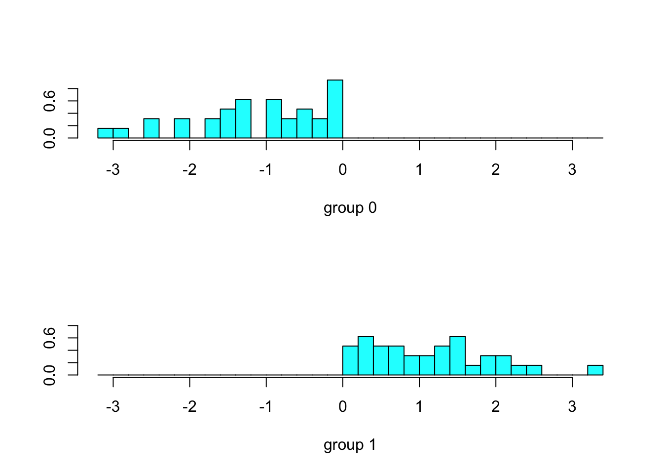
predict(dm)## $class
## [1] 1 1 1 1 1 1 1 1 0 1 1 1 0 1 1 1 0 1 0 1 1 1 1 1 1 0 1 1 1 1 1 1 0 0 0
## [36] 0 0 0 0 0 0 0 0 0 0 0 0 1 1 0 0 0 1 1 0 0 0 1 0 0 0 0 0 0
## Levels: 0 1
##
## $posterior
## 0 1
## 1 0.001299131 0.998700869
## 2 0.011196418 0.988803582
## 3 0.046608204 0.953391796
## 4 0.025364951 0.974635049
## 5 0.006459513 0.993540487
## 6 0.056366779 0.943633221
## 7 0.474976979 0.525023021
## 8 0.081379875 0.918620125
## 9 0.502094785 0.497905215
## 10 0.327329832 0.672670168
## 11 0.065547282 0.934452718
## 12 0.341547846 0.658452154
## 13 0.743464274 0.256535726
## 14 0.024815082 0.975184918
## 15 0.285683981 0.714316019
## 16 0.033598255 0.966401745
## 17 0.751098160 0.248901840
## 18 0.136470406 0.863529594
## 19 0.565743827 0.434256173
## 20 0.106256858 0.893743142
## 21 0.079260811 0.920739189
## 22 0.211287405 0.788712595
## 23 0.016145814 0.983854186
## 24 0.017916328 0.982083672
## 25 0.053361102 0.946638898
## 26 0.929799893 0.070200107
## 27 0.421467187 0.578532813
## 28 0.041196674 0.958803326
## 29 0.160473313 0.839526687
## 30 0.226165888 0.773834112
## 31 0.103861216 0.896138784
## 32 0.328218436 0.671781564
## 33 0.511514581 0.488485419
## 34 0.595293351 0.404706649
## 35 0.986761936 0.013238064
## 36 0.676574981 0.323425019
## 37 0.926833195 0.073166805
## 38 0.955066682 0.044933318
## 39 0.986527865 0.013472135
## 40 0.877497556 0.122502444
## 41 0.859503954 0.140496046
## 42 0.991731912 0.008268088
## 43 0.827209283 0.172790717
## 44 0.964180566 0.035819434
## 45 0.958246183 0.041753817
## 46 0.517839067 0.482160933
## 47 0.992279182 0.007720818
## 48 0.241060617 0.758939383
## 49 0.358987835 0.641012165
## 50 0.653092701 0.346907299
## 51 0.799810486 0.200189514
## 52 0.933218396 0.066781604
## 53 0.297058121 0.702941879
## 54 0.222809854 0.777190146
## 55 0.996971215 0.003028785
## 56 0.924919737 0.075080263
## 57 0.583330536 0.416669464
## 58 0.483663571 0.516336429
## 59 0.946886736 0.053113264
## 60 0.860202673 0.139797327
## 61 0.961358779 0.038641221
## 62 0.998027953 0.001972047
## 63 0.859521185 0.140478815
## 64 0.706002516 0.293997484
##
## $x
## LD1
## 1 3.346531869
## 2 2.256737828
## 3 1.520095227
## 4 1.837609440
## 5 2.536163975
## 6 1.419170979
## 7 0.050452000
## 8 1.220682015
## 9 -0.004220052
## 10 0.362761452
## 11 1.338252835
## 12 0.330587901
## 13 -0.535893942
## 14 1.848931516
## 15 0.461550632
## 16 1.691762218
## 17 -0.556253363
## 18 0.929165997
## 19 -0.133214789
## 20 1.072519927
## 21 1.235130454
## 22 0.663378952
## 23 2.069846547
## 24 2.016535392
## 25 1.448370738
## 26 -1.301200562
## 27 0.159527985
## 28 1.585103944
## 29 0.833369746
## 30 0.619515440
## 31 1.085352883
## 32 0.360730337
## 33 -0.023200674
## 34 -0.194348531
## 35 -2.171336821
## 36 -0.371720701
## 37 -1.278744604
## 38 -1.539410745
## 39 -2.162390029
## 40 -0.991628191
## 41 -0.912171192
## 42 -2.410924430
## 43 -0.788680213
## 44 -1.658362422
## 45 -1.578045708
## 46 -0.035952755
## 47 -2.445692660
## 48 0.577605329
## 49 0.291987243
## 50 -0.318630304
## 51 -0.697589676
## 52 -1.328191375
## 53 0.433803969
## 54 0.629224272
## 55 -2.919349215
## 56 -1.264701997
## 57 -0.169453310
## 58 0.032922090
## 59 -1.450847181
## 60 -0.915091388
## 61 -1.618696192
## 62 -3.135987051
## 63 -0.912243063
## 64 -0.44120800010.6.2 Confusion Matrix
This matrix shows some classification ability. Now we ask, what if the model has no classification ability, then what would the average confusion matrix look like? It’s easy to see that this would give a matrix that would assume no relation between the rows and columns, and the numbers in each cell would reflect the average number drawn based on row and column totals. In this case since the row and column totals are all 32, we get the following confusion matrix of no classification ability:
\[\begin{equation} E = \left[ \begin{array}{cc} 16 & 16\\ 16 & 16 \end{array} \right] \end{equation}\] The test statistic is the sum of squared normalized differences in the cells of both matrices, i.e., \[\begin{equation} \mbox{Test-Stat } = \sum_{i,j} \frac{[A_{ij} - E_{ij}]^2}{E_{ij}} \end{equation}\]We compute this in R.
A = matrix(c(27,5,5,27),2,2); print(A)## [,1] [,2]
## [1,] 27 5
## [2,] 5 27E = matrix(c(16,16,16,16),2,2); print(E)## [,1] [,2]
## [1,] 16 16
## [2,] 16 16test_stat = sum((A-E)^2/E); print(test_stat)## [1] 30.25print(1-pchisq(test_stat,1))## [1] 3.797912e-0810.7 Explanation of LDA
We assume two groups first for simplicity, 1 and 2. Assume a feature space \(x \in R^d\). Group 1 has \(n_1\) observations, and group 2 has \(n_2\) observations, i.e., tuples of dimension \(d\).
We want to find weights \(w \in R^d\) that will project each observation in each group onto a point \(z\) on a line, i.e.,
\[\begin{equation} z = w_1 x_1 + w_2 x_2 + ... + w_d x_d = w' x \end{equation}\]We want the \(z\) values of group 1 to be as far away as possible from that of group 2, accounting for the variation within and across groups.
The scatter within group \(j=1,2\) is defined as:
\[\begin{equation} S_j = \sum_{i=1}^{n_j} (z_{ji} - \bar{z}_j)^2 = \sum_{i=1}^{n_j} (w' x_{ji} - w'\bar{x}_j)^2 \end{equation}\]where \(\bar{z}_j\) is the scalar mean of \(z\) values for group \(j\), and \(\bar{x}_j\) is the mean of \(x\) values for group \(j\), and is of dimension \(d \times 1\).
We want to capture this scatter more formally, so we define
\[\begin{eqnarray} S_j = w' (x_{ji} - \bar{x}_j)(x_{ji} - \bar{x}_j)' w = w' V_j w \end{eqnarray}\]where we have defined \(V_j = (x_{ji} - \bar{x}_j)(x_{ji} - \bar{x}_j)'\) as the variation within group \(j\). We also define total within group variation as \(V_w = V_1 + V_2\). Think of \(V_j\) as a kind of covariance matrix of group \(j\).
We note that \(w\) is dimension \(d \times 1\), \((x_{ji} - \bar{x}_j)\) is dimension \(d \times n_j\), so that \(S_j\) is scalar.
We sum the within group scatter values to get the total within group variation, i.e.,
\[\begin{equation} w' (V_1 + V_2) w = w' V_w w \end{equation}\]For between group scatter, we get an analogous expression, i.e.,
\[\begin{equation} w' V_b w = w' (\bar{x}_1 - \bar{x}_2)(\bar{x}_1 - \bar{x}_2)' w \end{equation}\]where we note that \((\bar{x}_1 - \bar{x}_2)(\bar{x}_1 - \bar{x}_2)'\) is the between group covariance, and \(w\) is \((d \times 1)\), \((\bar{x}_1 - \bar{x}_2)\) is dimension \((d \times 1)\).
10.8 Fischer’s Discriminant
The Fischer linear discriminant approach is to maximize between group variation and minimize within group variation, i.e.,
\[\begin{equation} F = \frac{w' V_b w}{w' V_w w} \end{equation}\]Taking the vector derivative w.r.t. \(w\) to maximize, we get
\[\begin{equation} \frac{dF}{dw} = \frac{w' V_w w (2 V_b w) - w' V_b w (2 V_w w)}{(w' V_w w)^2} = {\bf 0} \end{equation}\] \[\begin{equation} V_b w - \frac{w' V_b w}{w' V_w w} V_w w = {\bf 0} \end{equation}\] \[\begin{equation} V_b w - F V_w w = {\bf 0} \end{equation}\] \[\begin{equation} V_w^{-1} V_b w - F w = {\bf 0} \end{equation}\]Rewrite this is an eigensystem and solve to get
\[\begin{eqnarray} Aw &=& \lambda w \\ w^* &=& V_w^{-1}(\bar{x}_1 - \bar{x}_2) \end{eqnarray}\]where \(A = V_w^{-1} V_b\), and \(\lambda=F\).
Note: An easy way to see how to solve for \(w^*\) is as follows. First, find the largest eigenvalue of matrix \(A\). Second, substitute that into the eigensystem and solve a system of \(d\) equations to get \(w\).
10.9 Generalizing number of groups
We proceed to \(k+1\) groups. Therefore now we need \(k\) discriminant vectors, i.e.,
\[\begin{equation} W = [w_1, w_2, ... , w_k] \in R^{d \times k} \end{equation}\]The Fischer discriminant generalizes to
\[\begin{equation} F = \frac{|W' V_b W|}{|W' V_w W|} \end{equation}\]where we now use the determinant as the numerator and denominator are no longer scalars. Note that between group variation is now \(V_w = V_1 + V_2 + ... + V_k\), and the denominator is the determinant of a \((k \times k)\) matrix.
The numerator is also the determinant of a \((k \times k)\) matrix, and
\[\begin{equation} V_b = \sum_{i=1}^k n_i (x_i - \bar{x}_i)(x_i - \bar{x}_i)' \end{equation}\]where \((x_i - \bar{x}_i)\) is of dimension \((d \times n_i)\), so that \(V_b\) is dimension \((d \times d)\).
y1 = rep(3,16)
y2 = rep(2,16)
y3 = rep(1,16)
y4 = rep(0,16)
y = c(y1,y2,y3,y4)
res = lda(y~x)
res
## Call:
## lda(y ~ x)
##
## Prior probabilities of groups:
## 0 1 2 3
## 0.25 0.25 0.25 0.25
##
## Group means:
## xPTS xREB xAST xTO xA.T xSTL xBLK xPF
## 0 61.43750 33.18750 11.93750 14.37500 0.888750 6.12500 1.8750 19.5000
## 1 62.78125 34.53125 11.00000 15.65625 0.782500 7.09375 2.8750 18.1875
## 2 70.31250 36.59375 13.50000 12.71875 1.094375 6.84375 3.1875 19.4375
## 3 73.87500 33.55625 14.55625 13.08125 1.145625 7.23125 3.0625 17.5000
## xFG xFT xX3P
## 0 0.4006875 0.7174375 0.3014375
## 1 0.3996250 0.6196250 0.3270000
## 2 0.4223750 0.7055625 0.3260625
## 3 0.4705000 0.7232500 0.3790000
##
## Coefficients of linear discriminants:
## LD1 LD2 LD3
## xPTS -0.03190376 -0.09589269 -0.03170138
## xREB 0.16962627 0.08677669 -0.11932275
## xAST 0.08820048 0.47175998 0.04601283
## xTO -0.20264768 -0.29407195 -0.02550334
## xA.T 0.02619042 -3.28901817 -1.42081485
## xSTL 0.23954511 -0.26327278 -0.02694612
## xBLK 0.05424102 -0.14766348 -0.17703174
## xPF 0.03678799 0.22610347 -0.09608475
## xFG 21.25583140 0.48722022 9.50234314
## xFT 5.42057568 6.39065311 2.72767409
## xX3P 1.98050128 -2.74869782 0.90901853
##
## Proportion of trace:
## LD1 LD2 LD3
## 0.6025 0.3101 0.0873y_pred = predict(res)$class
print(y_pred)## [1] 3 3 3 3 3 3 3 3 1 3 3 2 0 3 3 3 0 3 2 3 2 2 3 2 2 0 2 2 2 2 2 2 3 1 1
## [36] 1 0 1 1 1 1 1 1 1 1 1 0 2 2 0 0 0 0 2 0 0 2 0 1 0 1 1 0 0
## Levels: 0 1 2 3print(table(y,y_pred))## y_pred
## y 0 1 2 3
## 0 10 3 3 0
## 1 2 12 1 1
## 2 2 0 11 3
## 3 1 1 1 13print(chisq.test(table(y,y_pred)))## Warning in chisq.test(table(y, y_pred)): Chi-squared approximation may be
## incorrect##
## Pearson's Chi-squared test
##
## data: table(y, y_pred)
## X-squared = 78.684, df = 9, p-value = 2.949e-13The idea is that when we have 4 groups, we project each observation in the data into a 3-D space, which is then separated by hyperplanes to demarcate the 4 groups.
10.10 Eigen Systems
We now move on to understanding some properties of matrices that may be useful in classifying data or deriving its underlying components. We download Treasury interest rate date from the FRED website, http://research.stlouisfed.org/fred2/. I have placed the data in a file called “tryrates.txt”. Let’s read in the file.
rates = read.table("DSTMAA_data/tryrates.txt",header=TRUE)
print(names(rates))
## [1] "DATE" "FYGM3" "FYGM6" "FYGT1" "FYGT2" "FYGT3" "FYGT5" "FYGT7"
## [9] "FYGT10"print(head(rates))## DATE FYGM3 FYGM6 FYGT1 FYGT2 FYGT3 FYGT5 FYGT7 FYGT10
## 1 Jun-76 5.41 5.77 6.52 7.06 7.31 7.61 7.75 7.86
## 2 Jul-76 5.23 5.53 6.20 6.85 7.12 7.49 7.70 7.83
## 3 Aug-76 5.14 5.40 6.00 6.63 6.86 7.31 7.58 7.77
## 4 Sep-76 5.08 5.30 5.84 6.42 6.66 7.13 7.41 7.59
## 5 Oct-76 4.92 5.06 5.50 5.98 6.24 6.75 7.16 7.41
## 6 Nov-76 4.75 4.88 5.29 5.81 6.09 6.52 6.86 7.29Understanding eigenvalues and eigenvectors is best done visually. An excellent simple exposition is available at: http://setosa.io/ev/eigenvectors-and-eigenvalues/
A \(M \times M\) matrix \(A\) has attendant \(M\) eigenvectors \(V\) and eigenvalue \(\lambda\) if we can write
\[\begin{equation} \lambda V = A \; V \end{equation}\]Starting with matrix \(A\), the eigenvalue decomposition gives both \(V\) and \(\lambda\).
It turns out we can find \(M\) such eigenvalues and eigenvectors, as there is no unique solution to this equation. We also require that \(\lambda \neq 0\).
We may implement this in R as follows, setting matrix \(A\) equal to the covariance matrix of the rates of different maturities:
A = matrix(c(5,2,1,4),2,2)
E = eigen(A)
print(E)
## $values
## [1] 6 3
##
## $vectors
## [,1] [,2]
## [1,] 0.7071068 -0.4472136
## [2,] 0.7071068 0.8944272v1 = E$vectors[,1]
v2 = E$vectors[,2]
e1 = E$values[1]
e2 = E$values[2]
print(t(e1*v1))## [,1] [,2]
## [1,] 4.242641 4.242641print(A %*% v1)## [,1]
## [1,] 4.242641
## [2,] 4.242641print(t(e2*v2))## [,1] [,2]
## [1,] -1.341641 2.683282print(A %*% v2)## [,1]
## [1,] -1.341641
## [2,] 2.683282We see that the origin, eigenvalues and eigenvectors comprise \(n\) eigenspaces. The line from the origin through an eigenvector (i.e., a coordinate given by any one eigenvector) is called an “eigenspace”. All points on eigenspaces are themselves eigenvectors. These eigenpaces are dimensions in which the relationships between vectors in the matrix \(A\) load.
We may also think of the matrix \(A\) as an “operator” or function on vectors/matrices.
rates = as.matrix(rates[,2:9])
eigen(cov(rates))
## $values
## [1] 7.070996e+01 1.655049e+00 9.015819e-02 1.655911e-02 3.001199e-03
## [6] 2.145993e-03 1.597282e-03 8.562439e-04
##
## $vectors
## [,1] [,2] [,3] [,4] [,5] [,6]
## [1,] 0.3596990 -0.49201202 0.59353257 -0.38686589 0.34419189 -0.07045281
## [2,] 0.3581944 -0.40372601 0.06355170 0.20153645 -0.79515713 0.07823632
## [3,] 0.3875117 -0.28678312 -0.30984414 0.61694982 0.45913099 0.20442661
## [4,] 0.3753168 -0.01733899 -0.45669522 -0.19416861 -0.03906518 -0.46590654
## [5,] 0.3614653 0.13461055 -0.36505588 -0.41827644 0.06076305 -0.14203743
## [6,] 0.3405515 0.31741378 -0.01159915 -0.18845999 0.03366277 0.72373049
## [7,] 0.3260941 0.40838395 0.19017973 -0.05000002 -0.16835391 0.09196861
## [8,] 0.3135530 0.47616732 0.41174955 0.42239432 0.06132982 -0.42147082
## [,7] [,8]
## [1,] -0.04282858 0.03645143
## [2,] 0.15571962 -0.03744201
## [3,] -0.10492279 -0.16540673
## [4,] -0.30395044 0.54916644
## [5,] 0.45521861 -0.55849003
## [6,] 0.19935685 0.42773742
## [7,] -0.70469469 -0.39347299
## [8,] 0.35631546 0.13650940rcorr = cor(rates)
rcorr## FYGM3 FYGM6 FYGT1 FYGT2 FYGT3 FYGT5
## FYGM3 1.0000000 0.9975369 0.9911255 0.9750889 0.9612253 0.9383289
## FYGM6 0.9975369 1.0000000 0.9973496 0.9851248 0.9728437 0.9512659
## FYGT1 0.9911255 0.9973496 1.0000000 0.9936959 0.9846924 0.9668591
## FYGT2 0.9750889 0.9851248 0.9936959 1.0000000 0.9977673 0.9878921
## FYGT3 0.9612253 0.9728437 0.9846924 0.9977673 1.0000000 0.9956215
## FYGT5 0.9383289 0.9512659 0.9668591 0.9878921 0.9956215 1.0000000
## FYGT7 0.9220409 0.9356033 0.9531304 0.9786511 0.9894029 0.9984354
## FYGT10 0.9065636 0.9205419 0.9396863 0.9680926 0.9813066 0.9945691
## FYGT7 FYGT10
## FYGM3 0.9220409 0.9065636
## FYGM6 0.9356033 0.9205419
## FYGT1 0.9531304 0.9396863
## FYGT2 0.9786511 0.9680926
## FYGT3 0.9894029 0.9813066
## FYGT5 0.9984354 0.9945691
## FYGT7 1.0000000 0.9984927
## FYGT10 0.9984927 1.000000010.10.1 Intuition
So we calculated the eigenvalues and eigenvectors for the covariance matrix of the data. What does it really mean? Think of the covariance matrix as the summarization of the connections between the rates of different maturities in our data set. What we do not know is how many dimensions of commonality there are in these rates, and what is the relative importance of these dimensions. For each dimension of commonality, we wish to ask (a) how important is that dimension (the eigenvalue), and (b) the relative influence of that dimension on each rate (the values in the eigenvector). The most important dimension is the one with the highest eigenvalue, known as the principal eigenvalue, corresponding to which we have the principal eigenvector. It should be clear by now that the eigenvalue and its eigenvector are eigen pairs. It should also be intuitive why we call this the eigenvalue decomposition of a matrix.
10.11 Determinants
These functions of a matrix are also difficult to get an intuition for. But its best to think of the determinant as one possible function that returns the “sizing” of a matrix. More specifically, it relates to the volume of the space defined by the matrix. But not exactly, because it can also be negative, though the absolute size will give some sense of volume as well.
For example, let’s take the two-dimensional identity matrix, which defines the unit square.
a = matrix(0,2,2); diag(a) = 1
print(det(a))
## [1] 1print(det(2*a))## [1] 4We see immediately that when we multiply the matrix by 2, we get a determinant value that is four times the original, because the volume in two-dimensional space is area, and that has changed by 4. To verify, we’ll try the three-dimensional identity matrix.
a = matrix(0,3,3); diag(a) = 1
print(det(a))
## [1] 1print(det(2*a))## [1] 8Now we see that the orginal determinant has grown by \(2^3\) when all dimensions are doubled. We may also distort just one dimension, and see what happens.
a = matrix(0,2,2); diag(a) = 1
print(det(a))
## [1] 1a[2,2] = 2
print(det(a))## [1] 2That’s pretty self-explanatory!
10.12 Dimension Reduction: Factor Analysis and PCA
Factor analysis is the use of eigenvalue decomposition to uncover the underlying structure of the data. Given a data set of observations and explanatory variables, factor analysis seeks to achieve a decomposition with these two properties:
Obtain a reduced dimension set of explanatory variables, known as derived/extracted/discovered factors. Factors must be orthogonal, i.e., uncorrelated with each other.
Obtain data reduction, i.e., suggest a limited set of variables. Each such subset is a manifestation of an abstract underlying dimension.
These subsets are ordered in terms of their ability to explain the variation across observations.
See the article by Richard Darlington: http://www.psych.cornell.edu/Darlington/factor.htm, which is as good as any explanation one can get.
See also the article by Statsoft: http://www.statsoft.com/textbook/stfacan.html.
10.12.1 Notation
- Observations: \(y_i, i=1...N\).
- Original explanatory variables: \(x_{ik}, k=1...K\).
- Factors: \(F_j, j=1...M\).
- \(M < K\).
10.12.2 The Idea
As you can see in the rates data, there are eight different rates. If we wanted to model the underlying drivers of this system of rates, we could assume a separate driver for each one leading to \(K=8\) underlying factors. But the whole idea of factor analysis is to reduce the number of drivers that exist. So we may want to go with a smaller number of \(M < K\) factors.
The main concept here is to project the variables \(x \in R^{K}\) onto the reduced factor set \(F \in R^M\) such that we can explain most of the variables by the factors. Hence we are looking for a relation
\[\begin{equation} x = B F \end{equation}\]where \(B = \{b_{kj}\}\in R^{K \times M}\) is a matrix of factor loadings for the variables. Through matrix \(B\), \(x\) may be represented in smaller dimension \(M\). The entries in matrix \(B\) may be positive or negative. Negative loadings mean that the variable is negatively correlated with the factor. The whole idea is that we want to replace the relation of \(y\) to \(x\) with a relation of \(y\) to a reduced set \(F\).
Once we have the set of factors defined, then the \(N\) observations \(y\) may be expressed in terms of the factors through a factor score matrix \(A = \{a_{ij}\} \in R^{N \times M}\) as follows:
\[\begin{equation} y = A F \end{equation}\]Again, factor scores may be positive or negative. There are many ways in which such a transformation from variables to factors might be undertaken. We look at the most common one.
10.13 Principal Components Analysis (PCA)
In PCA, each component (factor) is viewed as a weighted combination of the other variables (this is not always the way factor analysis is implemented, but is certainly one of the most popular).
The starting point for PCA is the covariance matrix of the data. Essentially what is involved is an eigenvalue analysis of this matrix to extract the principal eigenvectors.
We can do the analysis using the R statistical package. Here is the sample session:
ncaa = read.table("DSTMAA_data/ncaa.txt",header=TRUE)
x = ncaa[4:14]
print(names(x))
## [1] "PTS" "REB" "AST" "TO" "A.T" "STL" "BLK" "PF" "FG" "FT" "X3P"result = princomp(x)
summary(result)## Importance of components:
## Comp.1 Comp.2 Comp.3 Comp.4
## Standard deviation 9.8747703 5.2870154 3.95773149 3.19879732
## Proportion of Variance 0.5951046 0.1705927 0.09559429 0.06244717
## Cumulative Proportion 0.5951046 0.7656973 0.86129161 0.92373878
## Comp.5 Comp.6 Comp.7 Comp.8
## Standard deviation 2.43526651 2.04505010 1.53272256 0.1314860827
## Proportion of Variance 0.03619364 0.02552391 0.01433727 0.0001055113
## Cumulative Proportion 0.95993242 0.98545633 0.99979360 0.9998991100
## Comp.9 Comp.10 Comp.11
## Standard deviation 1.062179e-01 6.591218e-02 3.007832e-02
## Proportion of Variance 6.885489e-05 2.651372e-05 5.521365e-06
## Cumulative Proportion 9.999680e-01 9.999945e-01 1.000000e+00screeplot(result)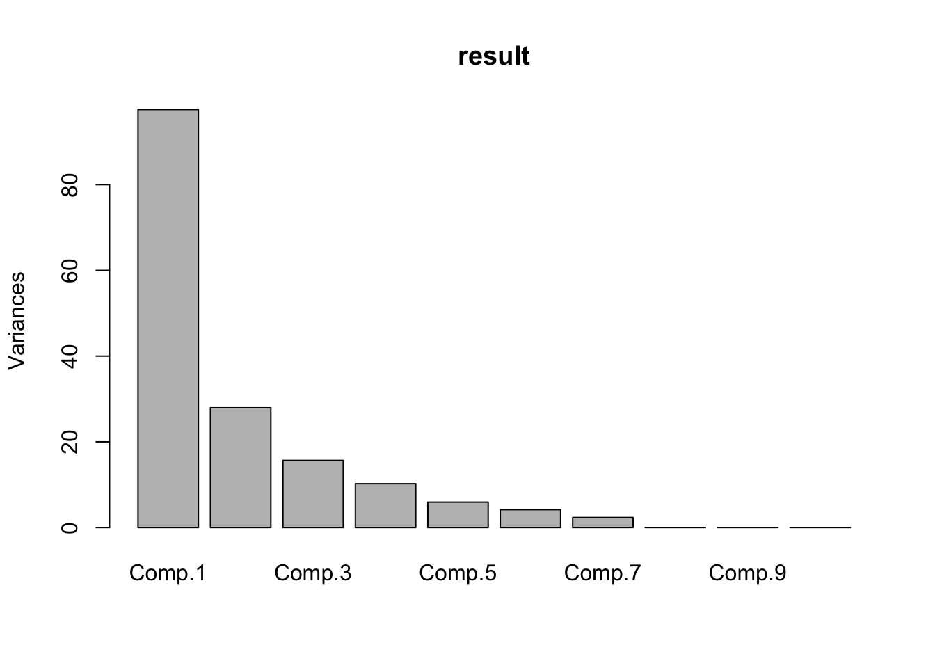
screeplot(result,type="lines")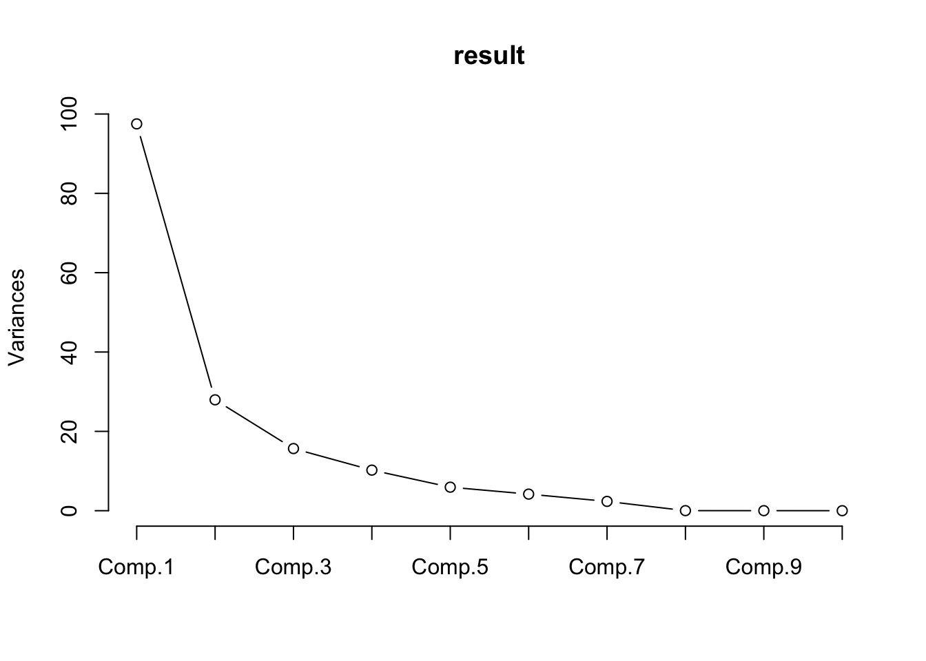
result$loadings##
## Loadings:
## Comp.1 Comp.2 Comp.3 Comp.4 Comp.5 Comp.6 Comp.7 Comp.8 Comp.9 Comp.10
## PTS 0.964 0.240
## REB 0.940 -0.316
## AST 0.257 -0.228 -0.283 -0.431 -0.778
## TO 0.194 -0.908 -0.116 0.313 -0.109
## A.T 0.712 0.642 0.262
## STL -0.194 0.205 0.816 0.498
## BLK 0.516 -0.849
## PF -0.110 -0.223 0.862 -0.364 -0.228
## FG
## FT 0.619 -0.762 0.175
## X3P -0.315 0.948
## Comp.11
## PTS
## REB
## AST
## TO
## A.T
## STL
## BLK
## PF
## FG -0.996
## FT
## X3P
##
## Comp.1 Comp.2 Comp.3 Comp.4 Comp.5 Comp.6 Comp.7 Comp.8
## SS loadings 1.000 1.000 1.000 1.000 1.000 1.000 1.000 1.000
## Proportion Var 0.091 0.091 0.091 0.091 0.091 0.091 0.091 0.091
## Cumulative Var 0.091 0.182 0.273 0.364 0.455 0.545 0.636 0.727
## Comp.9 Comp.10 Comp.11
## SS loadings 1.000 1.000 1.000
## Proportion Var 0.091 0.091 0.091
## Cumulative Var 0.818 0.909 1.000print(names(result))## [1] "sdev" "loadings" "center" "scale" "n.obs" "scores"
## [7] "call"result$sdev## Comp.1 Comp.2 Comp.3 Comp.4 Comp.5 Comp.6
## 9.87477028 5.28701542 3.95773149 3.19879732 2.43526651 2.04505010
## Comp.7 Comp.8 Comp.9 Comp.10 Comp.11
## 1.53272256 0.13148608 0.10621791 0.06591218 0.03007832biplot(result)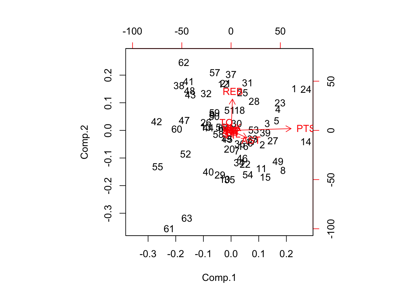
The alternative function prcomp returns the same stuff, but gives all the factor loadings immediately.
prcomp(x)## Standard deviations:
## [1] 9.95283292 5.32881066 3.98901840 3.22408465 2.45451793 2.06121675
## [7] 1.54483913 0.13252551 0.10705759 0.06643324 0.03031610
##
## Rotation:
## PC1 PC2 PC3 PC4 PC5
## PTS -0.963808450 -0.052962387 0.018398319 0.094091517 -0.240334810
## REB -0.022483140 -0.939689339 0.073265952 0.026260543 0.315515827
## AST -0.256799635 0.228136664 -0.282724110 -0.430517969 0.778063875
## TO 0.061658120 -0.193810802 -0.908005124 -0.115659421 -0.313055838
## A.T -0.021008035 0.030935414 0.035465079 -0.022580766 0.068308725
## STL -0.006513483 0.081572061 -0.193844456 0.205272135 0.014528901
## BLK -0.012711101 -0.070032329 0.035371935 0.073370876 -0.034410932
## PF -0.012034143 0.109640846 -0.223148274 0.862316681 0.364494150
## FG -0.003729350 0.002175469 -0.001708722 -0.006568270 -0.001837634
## FT -0.001210397 0.003852067 0.001793045 0.008110836 -0.019134412
## X3P -0.003804597 0.003708648 -0.001211492 -0.002352869 -0.003849550
## PC6 PC7 PC8 PC9 PC10
## PTS 0.029408534 -0.0196304356 0.0026169995 -0.004516521 0.004889708
## REB -0.040851345 -0.0951099200 -0.0074120623 0.003557921 -0.008319362
## AST -0.044767132 0.0681222890 0.0359559264 0.056106512 0.015018370
## TO 0.108917779 0.0864648004 -0.0416005762 -0.039363263 -0.012726102
## A.T -0.004846032 0.0061047937 -0.7122315249 -0.642496008 -0.262468560
## STL -0.815509399 -0.4981690905 0.0008726057 -0.008845999 -0.005846547
## BLK -0.516094006 0.8489313874 0.0023262933 -0.001364270 0.008293758
## PF 0.228294830 0.0972181527 0.0005835116 0.001302210 -0.001385509
## FG 0.004118140 0.0041758373 0.0848448651 -0.019610637 0.030860027
## FT -0.005525032 0.0001301938 -0.6189703010 0.761929615 -0.174641147
## X3P 0.001012866 0.0094289825 0.3151374823 0.038279107 -0.948194531
## PC11
## PTS 0.0037883918
## REB -0.0043776255
## AST 0.0058744543
## TO -0.0001063247
## A.T -0.0560584903
## STL -0.0062405867
## BLK 0.0013213701
## PF -0.0043605809
## FG -0.9956716097
## FT -0.0731951151
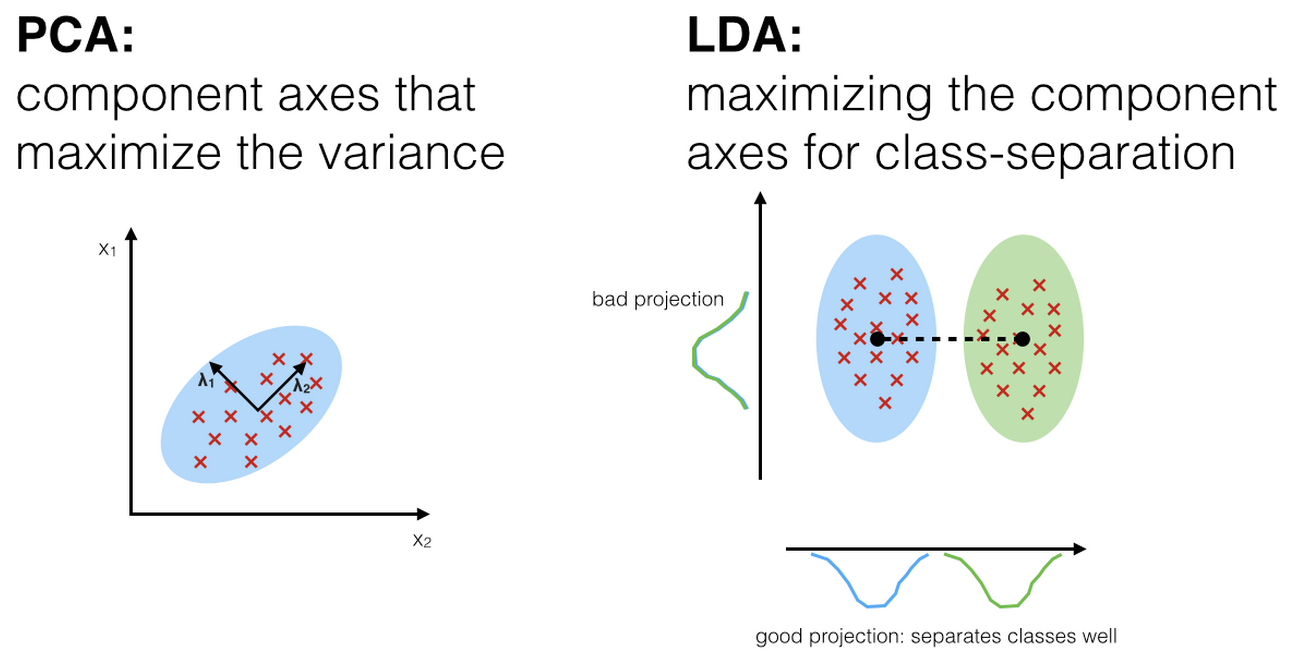
## X3P -0.003197629610.13.1 Difference between PCA and LDA
10.13.2 Application to Treasury Yield Curves
We had previously downloaded monthly data for constant maturity yields from June 1976 to December 2006. Here is the 3D plot. It shows the change in the yield curve over time for a range of maturities.
persp(rates,theta=30,phi=0,xlab="years",ylab="maturity",zlab="rates")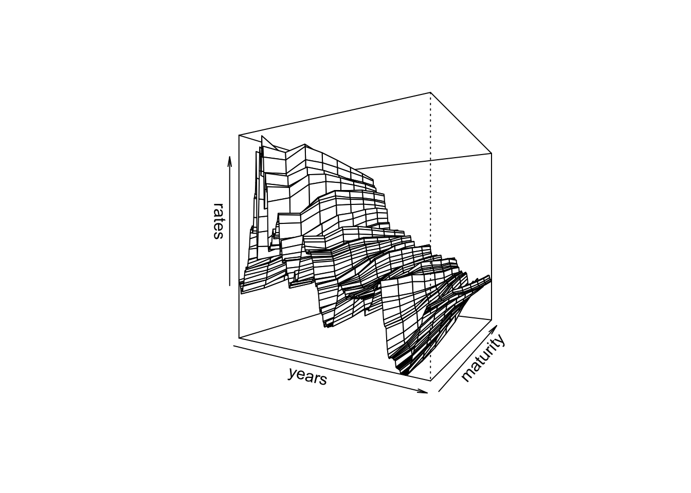
tryrates = read.table("DSTMAA_data/tryrates.txt",header=TRUE)
rates = as.matrix(tryrates[2:9])
result = princomp(rates)
result$loadings
##
## Loadings:
## Comp.1 Comp.2 Comp.3 Comp.4 Comp.5 Comp.6 Comp.7 Comp.8
## FYGM3 -0.360 -0.492 0.594 -0.387 0.344
## FYGM6 -0.358 -0.404 0.202 -0.795 -0.156
## FYGT1 -0.388 -0.287 -0.310 0.617 0.459 0.204 0.105 -0.165
## FYGT2 -0.375 -0.457 -0.194 -0.466 0.304 0.549
## FYGT3 -0.361 0.135 -0.365 -0.418 -0.142 -0.455 -0.558
## FYGT5 -0.341 0.317 -0.188 0.724 -0.199 0.428
## FYGT7 -0.326 0.408 0.190 -0.168 0.705 -0.393
## FYGT10 -0.314 0.476 0.412 0.422 -0.421 -0.356 0.137
##
## Comp.1 Comp.2 Comp.3 Comp.4 Comp.5 Comp.6 Comp.7 Comp.8
## SS loadings 1.000 1.000 1.000 1.000 1.000 1.000 1.000 1.000
## Proportion Var 0.125 0.125 0.125 0.125 0.125 0.125 0.125 0.125
## Cumulative Var 0.125 0.250 0.375 0.500 0.625 0.750 0.875 1.000result$sdev## Comp.1 Comp.2 Comp.3 Comp.4 Comp.5 Comp.6
## 8.39745750 1.28473300 0.29985418 0.12850678 0.05470852 0.04626171
## Comp.7 Comp.8
## 0.03991152 0.02922175summary(result)## Importance of components:
## Comp.1 Comp.2 Comp.3 Comp.4
## Standard deviation 8.397458 1.28473300 0.299854180 0.1285067846
## Proportion of Variance 0.975588 0.02283477 0.001243916 0.0002284667
## Cumulative Proportion 0.975588 0.99842275 0.999666666 0.9998951326
## Comp.5 Comp.6 Comp.7 Comp.8
## Standard deviation 5.470852e-02 4.626171e-02 3.991152e-02 2.922175e-02
## Proportion of Variance 4.140766e-05 2.960835e-05 2.203775e-05 1.181363e-05
## Cumulative Proportion 9.999365e-01 9.999661e-01 9.999882e-01 1.000000e+0010.13.3 Results
The results are interesting. We see that the loadings are large in the first three component vectors for all maturity rates. The loadings correspond to a classic feature of the yield curve, i.e., there are three components: level, slope, and curvature. Note that the first component has almost equal loadings for all rates that are all identical in sign. Hence, this is the level factor. The second component has negative loadings for the shorter maturity rates and positive loadings for the later maturity ones. Therefore, when this factor moves up, the short rates will go down, and the long rates will go up, resulting in a steepening of the yield curve. If the factor goes down, the yield curve will become flatter. Hence, the second principal component is clearly the slope factor. Examining the loadings of the third principal component should make it clear that the effect of this factor is to modulate the curvature or hump of the yield curve. Still, from looking at the results, it is clear that 97% of the common variation is explained by just the first factor, and a wee bit more by the next two. The resultant biplot shows the dominance of the main component.
biplot(result)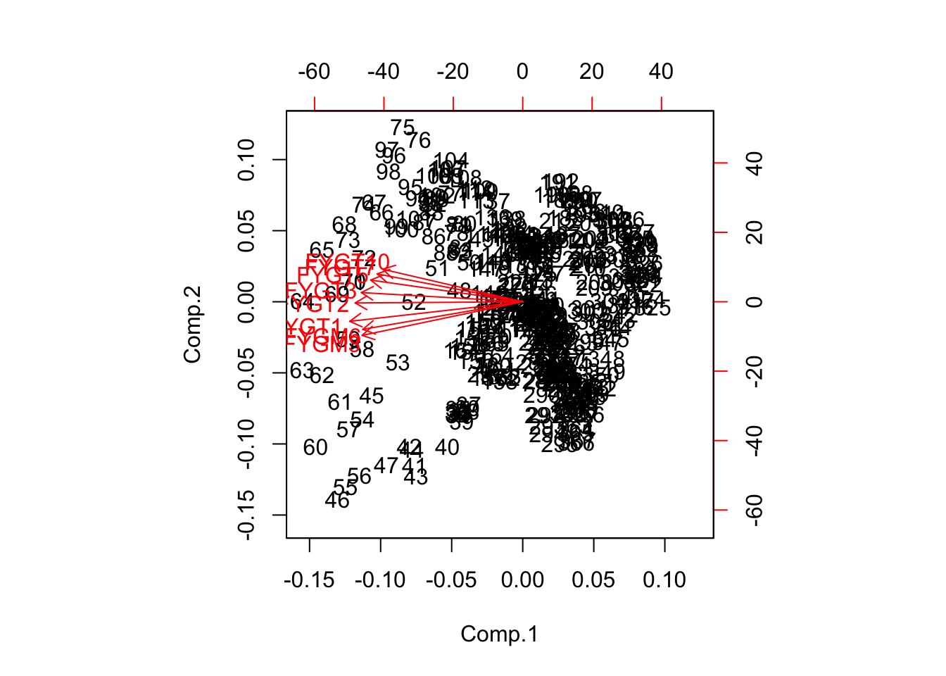
10.14 Difference between PCA and FA
The difference between PCA and FA is that for the purposes of matrix computations PCA assumes that all variance is common, with all unique factors set equal to zero; while FA assumes that there is some unique variance. Hence PCA may also be thought of as a subset of FA. The level of unique variance is dictated by the FA model which is chosen. Accordingly, PCA is a model of a closed system, while FA is a model of an open system. FA tries to decompose the correlation matrix into common and unique portions.
10.15 Factor Rotation
Finally, there are some times when the variables would load better on the factors if the factor system were to be rotated. This called factor rotation, and many times the software does this automatically.
Remember that we decomposed variables \(x\) as follows:
\[\begin{equation} x = B\;F + e \end{equation}\]where \(x\) is dimension \(K\), \(B \in R^{K \times M}\), \(F \in R^{M}\), and \(e\) is a \(K\)-dimension vector. This implies that
\[\begin{equation} Cov(x) = BB' + \psi \end{equation}\]Recall that \(B\) is the matrix of factor loadings. The system remains unchanged if \(B\) is replaced by \(BG\), where \(G \in R^{M \times M}\), and \(G\) is orthogonal. Then we call \(G\) a rotation of \(B\).
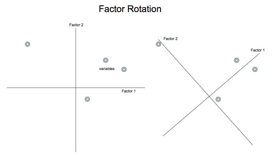
The idea of rotation is easier to see with the following diagram. Two conditions need to be satisfied: (a) The new axis (and the old one) should be orthogonal. (b) The difference in loadings on the factors by each variable must increase. In the diagram below we can see that the rotation has made the variables align better along the new axis system.
10.15.1 Using the factor analysis function
To illustrate, let’s undertake a factor analysis of the Treasury rates data. In R, we can implement it generally with the factanal command.
factanal(rates,2)##
## Call:
## factanal(x = rates, factors = 2)
##
## Uniquenesses:
## FYGM3 FYGM6 FYGT1 FYGT2 FYGT3 FYGT5 FYGT7 FYGT10
## 0.006 0.005 0.005 0.005 0.005 0.005 0.005 0.005
##
## Loadings:
## Factor1 Factor2
## FYGM3 0.843 0.533
## FYGM6 0.826 0.562
## FYGT1 0.793 0.608
## FYGT2 0.726 0.686
## FYGT3 0.681 0.731
## FYGT5 0.617 0.786
## FYGT7 0.579 0.814
## FYGT10 0.546 0.836
##
## Factor1 Factor2
## SS loadings 4.024 3.953
## Proportion Var 0.503 0.494
## Cumulative Var 0.503 0.997
##
## Test of the hypothesis that 2 factors are sufficient.
## The chi square statistic is 3556.38 on 13 degrees of freedom.
## The p-value is 0Notice how the first factor explains the shorter maturities better and the second factor explains the longer maturity rates. Hence, the two factors cover the range of maturities.
Note that the ability of the factors to separate the variables increases when we apply a factor rotation:
factanal(rates,2,rotation="promax")##
## Call:
## factanal(x = rates, factors = 2, rotation = "promax")
##
## Uniquenesses:
## FYGM3 FYGM6 FYGT1 FYGT2 FYGT3 FYGT5 FYGT7 FYGT10
## 0.006 0.005 0.005 0.005 0.005 0.005 0.005 0.005
##
## Loadings:
## Factor1 Factor2
## FYGM3 0.110 0.902
## FYGM6 0.174 0.846
## FYGT1 0.282 0.747
## FYGT2 0.477 0.560
## FYGT3 0.593 0.443
## FYGT5 0.746 0.284
## FYGT7 0.829 0.194
## FYGT10 0.895 0.118
##
## Factor1 Factor2
## SS loadings 2.745 2.730
## Proportion Var 0.343 0.341
## Cumulative Var 0.343 0.684
##
## Factor Correlations:
## Factor1 Factor2
## Factor1 1.000 -0.854
## Factor2 -0.854 1.000
##
## Test of the hypothesis that 2 factors are sufficient.
## The chi square statistic is 3556.38 on 13 degrees of freedom.
## The p-value is 0The factors have been reversed after the rotation. Now the first factor explains long rates and the second factor explains short rates.
If we want the time series of the factors, use the following command:
result = factanal(rates,2,scores="regression")
ts = result$scores
par(mfrow=c(2,1))
plot(ts[,1],type="l")
plot(ts[,2],type="l")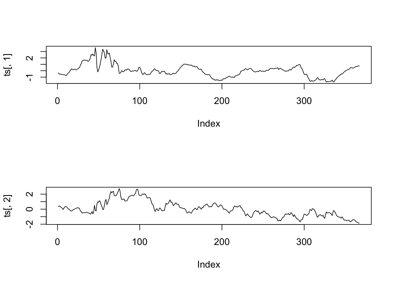
result$scores## Factor1 Factor2
## [1,] -0.355504878 0.3538523566
## [2,] -0.501355106 0.4219522836
## [3,] -0.543664379 0.3889362268
## [4,] -0.522169984 0.2906034115
## [5,] -0.566607393 0.1900987229
## [6,] -0.584273677 0.1158550772
## [7,] -0.617786769 -0.0509882532
## [8,] -0.624247257 0.1623048344
## [9,] -0.677009820 0.2997973824
## [10,] -0.733334654 0.3687408921
## [11,] -0.727719655 0.3139994343
## [12,] -0.500063146 0.2096808039
## [13,] -0.384131543 0.0410744861
## [14,] -0.295154982 0.0079262851
## [15,] -0.074469748 -0.0869377108
## [16,] 0.116075785 -0.2371344010
## [17,] 0.281023133 -0.2477845555
## [18,] 0.236661204 -0.1984323585
## [19,] 0.157626371 -0.0889735514
## [20,] 0.243074384 -0.0298846923
## [21,] 0.229996509 0.0114794387
## [22,] 0.147494917 0.0837694919
## [23,] 0.142866056 0.1429388300
## [24,] 0.217975571 0.1794260505
## [25,] 0.333131324 0.1632220682
## [26,] 0.427011092 0.1745390683
## [27,] 0.526015625 0.0105962505
## [28,] 0.930970981 -0.2759351140
## [29,] 1.099941917 -0.3067850535
## [30,] 1.531649405 -0.5218883427
## [31,] 1.612359229 -0.4795275595
## [32,] 1.674541369 -0.4768444035
## [33,] 1.628259706 -0.4725850979
## [34,] 1.666619753 -0.4812732821
## [35,] 1.607802989 -0.4160125641
## [36,] 1.637193575 -0.4306264237
## [37,] 1.453482425 -0.4656836872
## [38,] 1.525156467 -0.5096808367
## [39,] 1.674848519 -0.5570384352
## [40,] 2.049336334 -0.6730573078
## [41,] 2.541609184 -0.5458070626
## [42,] 2.420122121 -0.3166891875
## [43,] 2.598308192 -0.6327155757
## [44,] 2.391009307 -0.3356467032
## [45,] 2.311818441 0.5221104615
## [46,] 3.605474901 -0.1557021034
## [47,] 2.785430927 -0.2516679525
## [48,] 0.485057576 0.7228887760
## [49,] -0.189141617 0.9855640276
## [50,] 0.122281914 0.9105895503
## [51,] 0.511485539 1.1255567094
## [52,] 1.064745422 1.0034602577
## [53,] 1.750902392 0.6022272759
## [54,] 2.603592320 0.4009099335
## [55,] 3.355620751 -0.0481064328
## [56,] 3.096436233 -0.0475952393
## [57,] 2.790570579 0.4732116005
## [58,] 1.952978382 1.0839764053
## [59,] 2.007654491 1.3008974495
## [60,] 3.280609956 0.6027071203
## [61,] 2.650522546 0.7811051077
## [62,] 2.600300068 1.1915626752
## [63,] 2.766003209 1.4022416607
## [64,] 2.146320286 2.0370917324
## [65,] 1.479726566 2.3555071345
## [66,] 0.552668203 2.1652137124
## [67,] 0.556340456 2.3056213923
## [68,] 1.031484956 2.3872744033
## [69,] 1.723405950 1.8108125155
## [70,] 1.449614947 1.7709138593
## [71,] 1.460961876 1.7702209124
## [72,] 1.135992230 1.8967045582
## [73,] 1.135689418 2.2082173178
## [74,] 0.666878126 2.3873764566
## [75,] -0.383975947 2.7314819419
## [76,] -0.403354427 2.4378117276
## [77,] -0.261254207 1.6718118006
## [78,] 0.010954309 1.2752998691
## [79,] -0.092289703 1.3197429280
## [80,] -0.174691946 1.3083222077
## [81,] -0.097560278 1.3574900674
## [82,] 0.150646660 1.0910471461
## [83,] 0.121953667 1.0829765752
## [84,] 0.078801527 1.1050249969
## [85,] 0.278156097 1.2016627452
## [86,] 0.258501480 1.4588567047
## [87,] 0.210284188 1.6848813104
## [88,] 0.056036784 1.7137233052
## [89,] -0.118921800 1.7816790973
## [90,] -0.117431498 1.8372880351
## [91,] -0.040073664 1.8448115903
## [92,] -0.053649940 1.7738312784
## [93,] -0.027125996 1.8236531568
## [94,] 0.049919465 1.9851081358
## [95,] 0.029704916 2.1507133812
## [96,] -0.088880625 2.5931510323
## [97,] -0.047171830 2.6850656261
## [98,] 0.127458117 2.4718496073
## [99,] 0.538302707 1.8902746778
## [100,] 0.519981276 1.8260867038
## [101,] 0.287350732 1.8070920575
## [102,] -0.143185374 1.8168901486
## [103,] -0.477616832 1.9938013470
## [104,] -0.613354610 2.0298832121
## [105,] -0.412838433 1.9458918523
## [106,] -0.297013068 2.0396170842
## [107,] -0.510299939 1.9824043717
## [108,] -0.582920837 1.7520202839
## [109,] -0.620119822 1.4751073269
## [110,] -0.611872307 1.5171154200
## [111,] -0.547668692 1.5025027015
## [112,] -0.583785173 1.5461201027
## [113,] -0.495210980 1.4215226364
## [114,] -0.251451362 1.0449328603
## [115,] -0.082066002 0.6903391640
## [116,] -0.033194050 0.6316345737
## [117,] 0.182241740 0.2936690259
## [118,] 0.301423491 -0.1838473881
## [119,] 0.189478645 -0.3060949875
## [120,] 0.034277252 0.0074803060
## [121,] 0.031909353 0.0570923793
## [122,] 0.027356842 -0.1748564026
## [123,] -0.100678983 -0.1801001545
## [124,] -0.404727556 0.1406985128
## [125,] -0.424620066 0.1335285826
## [126,] -0.238905541 -0.0635401642
## [127,] -0.074664082 -0.2315185060
## [128,] -0.126155469 -0.2071550795
## [129,] -0.095540492 -0.1620034845
## [130,] -0.078865638 -0.1717327847
## [131,] -0.323056834 0.3504769061
## [132,] -0.515629047 0.7919922740
## [133,] -0.450893817 0.6472867847
## [134,] -0.549249387 0.7161373931
## [135,] -0.461526588 0.7850863426
## [136,] -0.477585081 1.0841412516
## [137,] -0.607936481 1.2313669640
## [138,] -0.602383745 0.9170263524
## [139,] -0.561466443 0.9439199208
## [140,] -0.440679406 0.7183641932
## [141,] -0.379694393 0.4646994387
## [142,] -0.448884489 0.5804226311
## [143,] -0.447585272 0.7304696952
## [144,] -0.394150535 0.8590552893
## [145,] -0.208356333 0.6731650551
## [146,] -0.089538357 0.6552198933
## [147,] 0.063317301 0.6517126106
## [148,] 0.251481083 0.3963555025
## [149,] 0.401325001 0.2069459108
## [150,] 0.566691007 0.1813057709
## [151,] 0.730739423 0.1753541513
## [152,] 0.828629006 0.1125881742
## [153,] 0.937069127 0.0763716514
## [154,] 1.044340934 0.0956119916
## [155,] 1.009393906 0.0347124400
## [156,] 1.003079712 -0.1255034699
## [157,] 1.017520561 -0.4004578618
## [158,] 0.932546637 -0.5165964072
## [159,] 0.952361490 -0.4406600026
## [160,] 0.875515542 -0.3342672213
## [161,] 0.869656935 -0.4237046276
## [162,] 0.888125852 -0.5145540230
## [163,] 0.861924343 -0.5076632865
## [164,] 0.738497876 -0.2536767792
## [165,] 0.691510554 -0.0954080233
## [166,] 0.741059090 -0.0544984271
## [167,] 0.614055561 0.1175151057
## [168,] 0.583992721 0.1208051871
## [169,] 0.655094889 -0.0609062254
## [170,] 0.585834845 -0.0430834033
## [171,] 0.348303688 0.1979721122
## [172,] 0.231869484 0.3331562586
## [173,] 0.200162810 0.2747729337
## [174,] 0.267236920 0.0828341446
## [175,] 0.210187651 -0.0004188853
## [176,] -0.109270296 0.2268927070
## [177,] -0.213761239 0.1965527314
## [178,] -0.348143133 0.4200966364
## [179,] -0.462961583 0.4705859027
## [180,] -0.578054300 0.5511131060
## [181,] -0.593897266 0.6647046884
## [182,] -0.606218752 0.6648334975
## [183,] -0.633747164 0.4861920257
## [184,] -0.595576784 0.3376759766
## [185,] -0.655205129 0.2879100847
## [186,] -0.877512941 0.3630640184
## [187,] -1.042216136 0.3097316247
## [188,] -1.210234114 0.4345481035
## [189,] -1.322308783 0.6532822938
## [190,] -1.277192666 0.7643285790
## [191,] -1.452808921 0.8312821327
## [192,] -1.487541641 0.8156176243
## [193,] -1.394870534 0.6686928699
## [194,] -1.479383323 0.4841365561
## [195,] -1.406886161 0.3273062670
## [196,] -1.492942737 0.3000294646
## [197,] -1.562195349 0.4406992406
## [198,] -1.516051602 0.5752479903
## [199,] -1.451353552 0.5211772634
## [200,] -1.501708646 0.4624047169
## [201,] -1.354991806 0.1902649452
## [202,] -1.228608089 -0.0070402815
## [203,] -1.267977350 -0.0029138561
## [204,] -1.230161999 0.0042656449
## [205,] -1.096818811 -0.0947205249
## [206,] -1.050883407 -0.1864794956
## [207,] -1.002987371 -0.2674961604
## [208,] -0.888334747 -0.4730245331
## [209,] -0.832011974 -0.5241786702
## [210,] -0.950806163 -0.2717874846
## [211,] -0.990904734 -0.2173246581
## [212,] -1.025888696 -0.2110302502
## [213,] -0.961207504 -0.1336593297
## [214,] -1.008873152 0.1426874706
## [215,] -1.066127710 0.4267411899
## [216,] -0.832669187 0.3633991700
## [217,] -0.804268297 0.3062188682
## [218,] -0.775554360 0.3751582494
## [219,] -0.654699498 0.2680646665
## [220,] -0.655827369 0.3622377616
## [221,] -0.572138953 0.4346262554
## [222,] -0.446528852 0.4693814204
## [223,] -0.065472508 0.2004701690
## [224,] -0.047390852 0.1708246675
## [225,] 0.033716643 -0.0546444756
## [226,] 0.090511779 -0.2360703511
## [227,] 0.096712210 -0.3211426773
## [228,] 0.263153818 -0.6427860627
## [229,] 0.327938463 -0.8977202535
## [230,] 0.227009433 -0.7738217993
## [231,] 0.146847582 -0.6164082349
## [232,] 0.217408892 -0.7820706869
## [233,] 0.303059068 -0.9119089249
## [234,] 0.346164990 -1.0156070316
## [235,] 0.344495268 -1.0989068333
## [236,] 0.254605496 -1.0839365333
## [237,] 0.076434520 -0.9212083749
## [238,] -0.038930459 -0.5853123528
## [239,] -0.124579936 -0.3899503999
## [240,] -0.184503898 -0.2610908904
## [241,] -0.195782588 -0.1682655163
## [242,] -0.130929970 -0.2396129985
## [243,] -0.107305460 -0.3638191317
## [244,] -0.146037350 -0.2440039282
## [245,] -0.091759778 -0.4265627928
## [246,] 0.060904468 -0.6770486218
## [247,] -0.021981240 -0.5691143174
## [248,] -0.098778176 -0.3937451878
## [249,] -0.046565752 -0.4968429844
## [250,] -0.074221981 -0.3346834015
## [251,] -0.114633531 -0.2075481471
## [252,] -0.080181397 -0.3167544243
## [253,] -0.077245027 -0.4075464988
## [254,] 0.067095102 -0.6330318266
## [255,] 0.070287704 -0.6063439043
## [256,] 0.034358274 -0.6110384546
## [257,] 0.122570752 -0.7498264729
## [258,] 0.268350996 -0.9191662258
## [259,] 0.341928786 -0.9953776859
## [260,] 0.358493675 -1.1493486058
## [261,] 0.366995992 -1.1315765328
## [262,] 0.308211094 -1.0360637068
## [263,] 0.296634032 -1.0283183308
## [264,] 0.333921857 -1.0482262664
## [265,] 0.399654634 -1.1547504178
## [266,] 0.384082293 -1.1639983135
## [267,] 0.398207702 -1.2498402091
## [268,] 0.458285541 -1.5595689354
## [269,] 0.190961643 -1.5179769824
## [270,] 0.312795727 -1.4594244181
## [271,] 0.384110006 -1.5668180503
## [272,] 0.289341234 -1.4408671342
## [273,] 0.219416836 -1.2581560002
## [274,] 0.109564976 -1.0724088237
## [275,] 0.062406607 -1.0647289538
## [276,] -0.003233728 -0.8644137409
## [277,] -0.073271391 -0.6429640308
## [278,] -0.092114043 -0.6751620268
## [279,] -0.035775597 -0.6458887585
## [280,] -0.018356448 -0.6699793136
## [281,] -0.024265930 -0.5752117330
## [282,] 0.169113471 -0.7594497105
## [283,] 0.196907611 -0.6785741261
## [284,] 0.099214208 -0.4437077861
## [285,] 0.261745559 -0.5584470428
## [286,] 0.459835499 -0.7964931207
## [287,] 0.571275193 -0.9824797396
## [288,] 0.480016597 -0.7239083896
## [289,] 0.584006730 -0.9603237689
## [290,] 0.684635191 -1.0869791122
## [291,] 0.854501019 -1.2873287505
## [292,] 0.829639616 -1.3076896394
## [293,] 0.904390403 -1.4233854975
## [294,] 0.965487586 -1.4916665856
## [295,] 0.939437320 -1.6964516427
## [296,] 0.503593382 -1.4775751602
## [297,] 0.360893182 -1.3829316066
## [298,] 0.175593148 -1.3465999103
## [299,] -0.251176076 -0.9627487991
## [300,] -0.539075038 -0.6634413175
## [301,] -0.599350551 -0.6725569082
## [302,] -0.556412743 -0.7281211894
## [303,] -0.540217609 -0.8466812382
## [304,] -0.862343566 -0.7743682184
## [305,] -1.120682354 -0.6757445700
## [306,] -1.332197920 -0.4766963100
## [307,] -1.635390509 -0.0574670942
## [308,] -1.640813369 -0.0797300906
## [309,] -1.529734133 -0.1952548992
## [310,] -1.611895694 0.0685046158
## [311,] -1.620979516 0.0300820065
## [312,] -1.611657565 -0.0337932009
## [313,] -1.521101087 -0.2270269452
## [314,] -1.434980209 -0.4497880483
## [315,] -1.283417015 -0.7628290825
## [316,] -1.072346961 -1.0683534564
## [317,] -1.140637580 -1.0104383462
## [318,] -1.395549643 -0.7734735074
## [319,] -1.415043289 -0.7733548411
## [320,] -1.454986296 -0.7501208892
## [321,] -1.388833790 -0.8644898171
## [322,] -1.365505724 -0.9246379945
## [323,] -1.439150405 -0.8129456121
## [324,] -1.262015053 -1.1101810729
## [325,] -1.242212525 -1.2288228293
## [326,] -1.575868993 -0.7274654884
## [327,] -1.776113351 -0.3592139365
## [328,] -1.688938879 -0.5119478063
## [329,] -1.700951156 -0.4941221141
## [330,] -1.694672567 -0.4605841099
## [331,] -1.702468087 -0.4640479153
## [332,] -1.654904379 -0.5634761675
## [333,] -1.601784931 -0.6271607888
## [334,] -1.459084170 -0.8494350933
## [335,] -1.690953476 -0.4241288061
## [336,] -1.763251101 -0.1746603929
## [337,] -1.569093305 -0.2888010297
## [338,] -1.408665012 -0.5098879003
## [339,] -1.249641136 -0.7229902408
## [340,] -1.064271255 -0.9142618698
## [341,] -0.969933254 -0.9878591695
## [342,] -0.829422105 -1.0259461991
## [343,] -0.746049960 -1.0573799245
## [344,] -0.636393008 -1.1066676094
## [345,] -0.496790978 -1.1981395438
## [346,] -0.526818274 -1.0157822994
## [347,] -0.406273939 -1.1747944777
## [348,] -0.266428973 -1.3514185013
## [349,] -0.152652610 -1.4757833223
## [350,] -0.063065136 -1.4551322378
## [351,] 0.044113220 -1.4821790342
## [352,] 0.083554485 -1.5531582261
## [353,] 0.149851616 -1.4719167589
## [354,] 0.214089933 -1.4732795716
## [355,] 0.267359067 -1.5397675087
## [356,] 0.433101487 -1.6864685717
## [357,] 0.487372036 -1.6363593913
## [358,] 0.465044913 -1.5603091398
## [359,] 0.407435603 -1.4222412386
## [360,] 0.424439377 -1.3921872057
## [361,] 0.500793195 -1.4233665943
## [362,] 0.590547206 -1.5031899730
## [363,] 0.658037559 -1.6520855175
## [364,] 0.663797018 -1.7232186290
## [365,] 0.700576947 -1.7445853037
## [366,] 0.780491234 -1.8529250191
## [367,] 0.747690062 -1.8487246210