Chapter 3 Open Source: R Programming
“Walking on water and developing software from a specification are easy if both are frozen” – Edward V. Berard
3.1 Got R?
In this chapter, we develop some expertise in using the R statistical package. See the manual https://cran.r-project.org/doc/manuals/r-release/R-intro.pdf on the R web site. Work through Appendix A, at least the first page. Also see Grant Farnsworth’s document “Econometrics in R”: https://cran.r-project.org/doc/contrib/Farnsworth-EconometricsInR.pdf.
There is also a great book that I personally find to be of very high quality, titled “The Art of R Programming” by Norman Matloff.
You can easily install the R programming language, which is a very useful tool for Machine Learning. See: http://en.wikipedia.org/wiki/Machine_learning
Get R from: http://www.r-project.org/ (download and install it).
If you want to use R in IDE mode, download RStudio: http://www.rstudio.com.
Here is qa quick test to make sure your installation of R is working along with graphics capabilities.
#PLOT HISTOGRAM FROM STANDARD NORMAL RANDOM NUMBERS
x = rnorm(1000000)
hist(x,50)
grid(col="blue",lwd=2)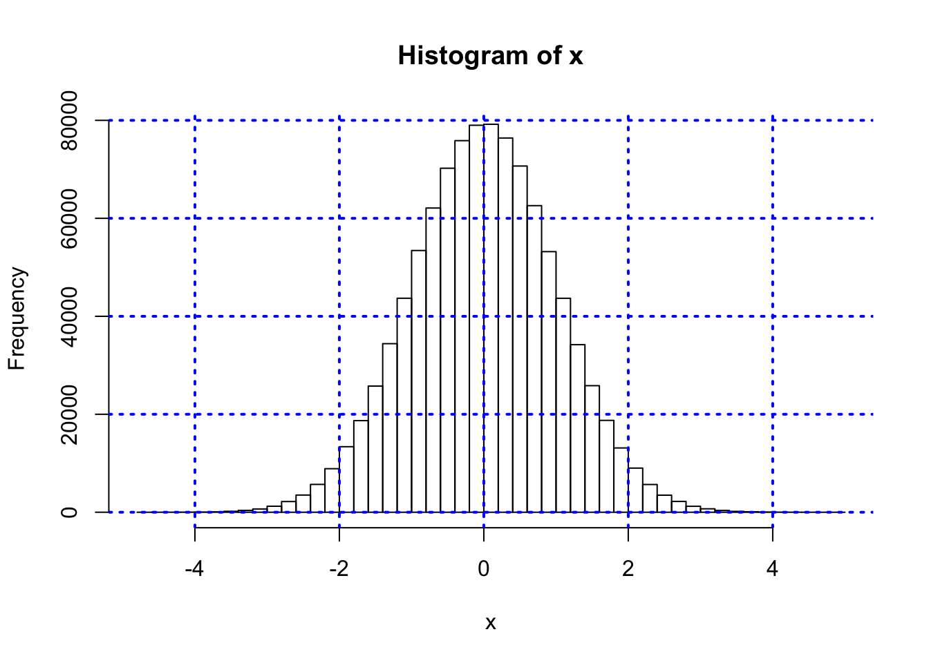
3.1.1 System Commands
If you want to directly access the system you can issue system commands as follows:
#SYSTEM COMMANDS
#The following command will show the files in the directory which are notebooks.
print(system("ls -lt"))  #This command will not work in the notebook.
## [1] 03.2 Loading Data
To get started, we need to grab some data. Go to Yahoo! Finance and download some historical data in an Excel spreadsheet, re-sort it into chronological order, then save it as a CSV file. Read the file into R as follows.
#READ IN DATA FROM CSV FILE
data = read.csv("DSTMAA_data/goog.csv",header=TRUE)
print(head(data))
## Date Open High Low Close Volume Adj.Close
## 1 2011-04-06 572.18 575.16 568.00 574.18 2668300 574.18
## 2 2011-04-05 581.08 581.49 565.68 569.09 6047500 569.09
## 3 2011-04-04 593.00 594.74 583.10 587.68 2054500 587.68
## 4 2011-04-01 588.76 595.19 588.76 591.80 2613200 591.80
## 5 2011-03-31 583.00 588.16 581.74 586.76 2029400 586.76
## 6 2011-03-30 584.38 585.50 580.58 581.84 1422300 581.84m = length(data)
n = length(data[,1])
print(c("Number of columns = ",m))## [1] "Number of columns = " "7"print(c("Length of data series = ",n))## [1] "Length of data series = " "1671"#REVERSE ORDER THE DATA (Also get some practice with a for loop)
for (j in 1:m) {
data[,j] = rev(data[,j])
}
print(head(data))## Date Open High Low Close Volume Adj.Close
## 1 2004-08-19 100.00 104.06 95.96 100.34 22351900 100.34
## 2 2004-08-20 101.01 109.08 100.50 108.31 11428600 108.31
## 3 2004-08-23 110.75 113.48 109.05 109.40 9137200 109.40
## 4 2004-08-24 111.24 111.60 103.57 104.87 7631300 104.87
## 5 2004-08-25 104.96 108.00 103.88 106.00 4598900 106.00
## 6 2004-08-26 104.95 107.95 104.66 107.91 3551000 107.91stkp = as.matrix(data[,7])
plot(stkp,type="l",col="blue")
grid(lwd=2)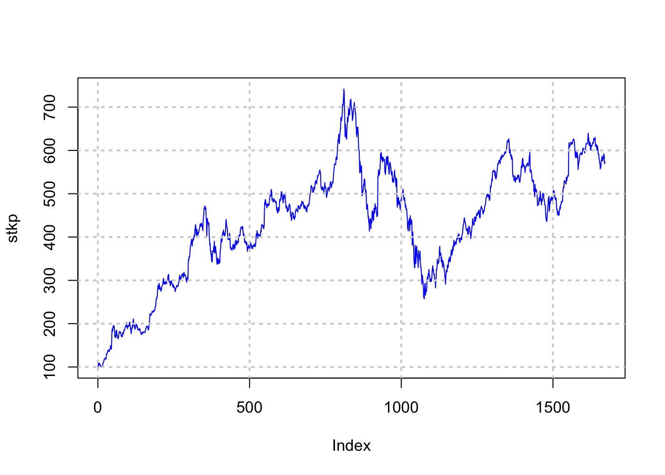
The last command reverses the sequence of the data if required.
3.3 Getting External Stock Data
We can do the same data set up exercise for financial data using the quantmod package.
Note: to install a package you can use the drop down menus on Windows and Mac operating systems, and use a package installer on Linux. Or issue the following command:
install.packages("quantmod")Now we move on to using this package for one stock.
#USE THE QUANTMOD PACKAGE TO GET STOCK DATA
library(quantmod)
## Loading required package: xts## Loading required package: zoo##
## Attaching package: 'zoo'## The following objects are masked from 'package:base':
##
## as.Date, as.Date.numeric## Loading required package: TTR## Loading required package: methods## Version 0.4-0 included new data defaults. See ?getSymbols.getSymbols("IBM")## As of 0.4-0, 'getSymbols' uses env=parent.frame() and
## auto.assign=TRUE by default.
##
## This behavior will be phased out in 0.5-0 when the call will
## default to use auto.assign=FALSE. getOption("getSymbols.env") and
## getOptions("getSymbols.auto.assign") are now checked for alternate defaults
##
## This message is shown once per session and may be disabled by setting
## options("getSymbols.warning4.0"=FALSE). See ?getSymbols for more details.## [1] "IBM"chartSeries(IBM)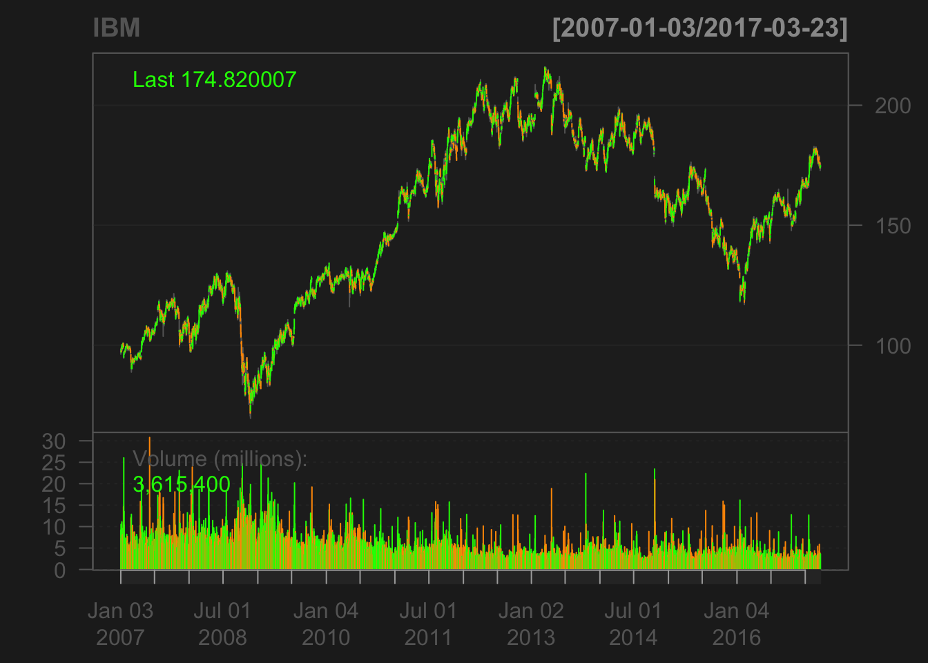
Let’s take a quick look at the data.
head(IBM)## IBM.Open IBM.High IBM.Low IBM.Close IBM.Volume IBM.Adjusted
## 2007-01-03 97.18 98.40 96.26 97.27 9196800 77.73997
## 2007-01-04 97.25 98.79 96.88 98.31 10524500 78.57116
## 2007-01-05 97.60 97.95 96.91 97.42 7221300 77.85985
## 2007-01-08 98.50 99.50 98.35 98.90 10340000 79.04270
## 2007-01-09 99.08 100.33 99.07 100.07 11108200 79.97778
## 2007-01-10 98.50 99.05 97.93 98.89 8744800 79.03470Extract the dates using pipes (we will see this in more detail later).
library(magrittr)
dts = IBM %>% as.data.frame %>% row.names
dts %>% head %>% print
## [1] "2007-01-03" "2007-01-04" "2007-01-05" "2007-01-08" "2007-01-09"
## [6] "2007-01-10"dts %>% length %>% print## [1] 2574Plot the data.
stkp = as.matrix(IBM$IBM.Adjusted)
rets = diff(log(stkp))
dts = as.Date(dts)
plot(dts,stkp,type="l",col="blue",xlab="Years",ylab="Stock Price of IBM")
grid(lwd=2)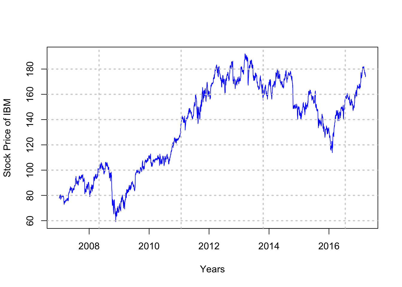
Summarize the data.
#DESCRIPTIVE STATS
summary(IBM)
## Index IBM.Open IBM.High IBM.Low
## Min. :2007-01-03 Min. : 72.74 Min. : 76.98 Min. : 69.5
## 1st Qu.:2009-07-23 1st Qu.:122.59 1st Qu.:123.97 1st Qu.:121.5
## Median :2012-02-09 Median :155.01 Median :156.29 Median :154.0
## Mean :2012-02-11 Mean :151.07 Mean :152.32 Mean :150.0
## 3rd Qu.:2014-09-02 3rd Qu.:183.52 3rd Qu.:184.77 3rd Qu.:182.4
## Max. :2017-03-23 Max. :215.38 Max. :215.90 Max. :214.3
## IBM.Close IBM.Volume IBM.Adjusted
## Min. : 71.74 Min. : 1027500 Min. : 59.16
## 1st Qu.:122.70 1st Qu.: 3615825 1st Qu.:101.43
## Median :155.38 Median : 4979650 Median :143.63
## Mean :151.19 Mean : 5869075 Mean :134.12
## 3rd Qu.:183.54 3rd Qu.: 7134350 3rd Qu.:166.28
## Max. :215.80 Max. :30770700 Max. :192.08Compute risk (volatility).
#STOCK VOLATILITY
sigma_daily = sd(rets)
sigma_annual = sigma_daily*sqrt(252)
print(sigma_annual)
## [1] 0.2234349print(c("Sharpe ratio = ",mean(rets)*252/sigma_annual))## [1] "Sharpe ratio = " "0.355224144170446"We may also use the package to get data for more than one stock.
library(quantmod)
getSymbols(c("GOOG","AAPL","CSCO","IBM"))
## [1] "GOOG" "AAPL" "CSCO" "IBM"We now go ahead and concatenate columns of data into one stock data set.
goog = as.numeric(GOOG[,6])
aapl = as.numeric(AAPL[,6])
csco = as.numeric(CSCO[,6])
ibm = as.numeric(IBM[,6])
stkdata = cbind(goog,aapl,csco,ibm)
dim(stkdata)
## [1] 2574 4Now, compute daily returns. This time, we do log returns in continuous-time. The mean returns are:
n = dim(stkdata)[1]
rets = log(stkdata[2:n,]/stkdata[1:(n-1),])
colMeans(rets)
## goog aapl csco ibm
## 0.0004869421 0.0009962588 0.0001426355 0.0003149582We can also compute the covariance matrix and correlation matrix:
cv = cov(rets)
print(cv,2)
## goog aapl csco ibm
## goog 0.00034 0.00020 0.00017 0.00012
## aapl 0.00020 0.00042 0.00019 0.00014
## csco 0.00017 0.00019 0.00036 0.00015
## ibm 0.00012 0.00014 0.00015 0.00020cr = cor(rets)
print(cr,4)## goog aapl csco ibm
## goog 1.0000 0.5342 0.4984 0.4627
## aapl 0.5342 1.0000 0.4840 0.4743
## csco 0.4984 0.4840 1.0000 0.5711
## ibm 0.4627 0.4743 0.5711 1.0000Notice the print command allows you to choose the number of significant digits (in this case 4). Also, as expected the four return time series are positively correlated with each other.
3.4 Data Frames
Data frames are the most essential data structure in the R programming language. One may think of a data frame as simply a spreadsheet. In fact you can view it as such with the following command.
View(data)However, data frames in R are much more than mere spreadsheets, which is why Excel will never trump R in the hanlding and analysis of data, except for very small applications on small spreadsheets. One may also think of data frames as databases, and there are many commands that we may use that are database-like, such as joins, merges, filters, selections, etc. Indeed, packages such as dplyr and data.table are designed to make these operations seamless, and operate efficiently on big data, where the number of observations (rows) are of the order of hundreds of millions.
Data frames can be addressed by column names, so that we do not need to remember column numbers specifically. If you want to find the names of all columns in a data frame, the names function does the trick. To address a chosen column, append the column name to the data frame using the “$” connector, as shown below.
#THIS IS A DATA FRAME AND CAN BE REFERENCED BY COLUMN NAMES
print(names(data))
## [1] "Date" "Open" "High" "Low" "Close" "Volume"
## [7] "Adj.Close"print(head(data$Close))## [1] 100.34 108.31 109.40 104.87 106.00 107.91The command printed out the first few observations in the column “Close”. All variables and functions in R are “objects”, and you are well-served to know the object type, because objects have properties and methods apply differently to objects of various types. Therefore, to check an object type, use the class function.
class(data)## [1] "data.frame"To obtain descriptive statistics on the data variables in a data frame, the summary function is very handy.
#DESCRIPTIVE STATISTICS
summary(data)
## Date Open High Low
## 2004-08-19: 1 Min. : 99.19 Min. :101.7 Min. : 95.96
## 2004-08-20: 1 1st Qu.:353.79 1st Qu.:359.5 1st Qu.:344.25
## 2004-08-23: 1 Median :457.57 Median :462.2 Median :452.42
## 2004-08-24: 1 Mean :434.70 Mean :439.7 Mean :429.15
## 2004-08-25: 1 3rd Qu.:532.62 3rd Qu.:537.2 3rd Qu.:526.15
## 2004-08-26: 1 Max. :741.13 Max. :747.2 Max. :725.00
## (Other) :1665
## Close Volume Adj.Close
## Min. :100.0 Min. : 858700 Min. :100.0
## 1st Qu.:353.5 1st Qu.: 3200350 1st Qu.:353.5
## Median :457.4 Median : 5028000 Median :457.4
## Mean :434.4 Mean : 6286021 Mean :434.4
## 3rd Qu.:531.6 3rd Qu.: 7703250 3rd Qu.:531.6
## Max. :741.8 Max. :41116700 Max. :741.8
## Let’s take a given column of data and perform some transformations on it. We can also plot the data, with some arguments for look and feel, using the plot function.
#USING A PARTICULAR COLUMN
stkp = data$Adj.Close
dt = data$Date
print(c("Length of stock series = ",length(stkp)))
## [1] "Length of stock series = " "1671"#Ln of differenced stk prices gives continuous returns
rets = diff(log(stkp)) #diff() takes first differences
print(c("Length of return series = ",length(rets)))## [1] "Length of return series = " "1670"print(head(rets))## [1] 0.07643307 0.01001340 -0.04228940 0.01071761 0.01785845 -0.01644436plot(rets,type="l",col="blue")
In case you want more descriptive statistics than provided by the summary function, then use an appropriate package. We may be interested in the higher-order moments, and we use the moments package for this.
print(summary(rets))## Min. 1st Qu. Median Mean 3rd Qu. Max.
## -0.1234000 -0.0092080 0.0007246 0.0010450 0.0117100 0.1823000Compute the daily and annualized standard deviation of returns.
r_sd = sd(rets)
r_sd_annual = r_sd*sqrt(252)
print(c(r_sd,r_sd_annual))
## [1] 0.02266823 0.35984704#What if we take the stdev of annualized returns?
print(sd(rets*252))## [1] 5.712395#Huh?
print(sd(rets*252))/252## [1] 5.712395## [1] 0.02266823print(sd(rets*252))/sqrt(252)## [1] 5.712395## [1] 0.359847Notice the interesting use of the print function here. The variance is easy as well.
#Variance
r_var = var(rets)
r_var_annual = var(rets)*252
print(c(r_var,r_var_annual))
## [1] 0.0005138488 0.12948989533.5 Higher-Order Moments
Skewness and kurtosis are key moments that arise in all return distributions. We need a different library in R for these. We use the moments library.
\[\begin{equation} \mbox{Skewness} = \frac{E[(X-\mu)^3]}{\sigma^{3}} \end{equation}\]Skewness means one tail is fatter than the other (asymmetry). Fatter right (left) tail implies positive (negative) skewness.
\[\begin{equation} \mbox{Kurtosis} = \frac{E[(X-\mu)^4]}{\sigma^{4}} \end{equation}\]Kurtosis means both tails are fatter than with a normal distribution.
#HIGHER-ORDER MOMENTS
library(moments)
hist(rets,50)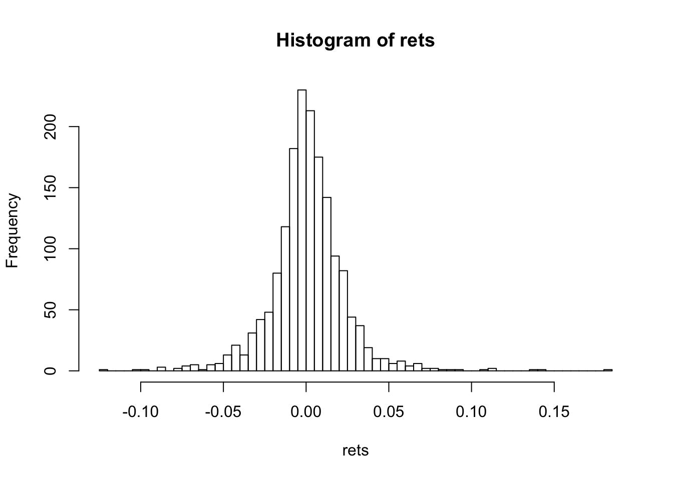
print(c("Skewness=",skewness(rets)))## [1] "Skewness=" "0.487479193296115"print(c("Kurtosis=",kurtosis(rets)))## [1] "Kurtosis=" "9.95591572103069"For the normal distribution, skewness is zero, and kurtosis is 3. Kurtosis minus three is denoted “excess kurtosis”.
skewness(rnorm(1000000))## [1] 0.001912514kurtosis(rnorm(1000000))## [1] 2.995332What is the skewness and kurtosis of the stock index (S&P500)?
3.6 Reading space delimited files
Often the original data is in a space delimited file, not a comma separated one, in which case the read.table function is appropriate.
#READ IN MORE DATA USING SPACE DELIMITED FILE
data = read.table("DSTMAA_data/markowitzdata.txt",header=TRUE)
print(head(data))
## X.DATE SUNW MSFT IBM CSCO AMZN
## 1 20010102 -0.087443948 0.000000000 -0.002205882 -0.129084975 -0.10843374
## 2 20010103 0.297297299 0.105187319 0.115696386 0.240150094 0.26576576
## 3 20010104 -0.060606062 0.010430248 -0.015191546 0.013615734 -0.11743772
## 4 20010105 -0.096774191 0.014193549 0.008718981 -0.125373140 -0.06048387
## 5 20010108 0.006696429 -0.003816794 -0.004654255 -0.002133106 0.02575107
## 6 20010109 0.044345897 0.058748405 -0.010688043 0.015818726 0.09623431
## mktrf smb hml rf
## 1 -0.0345 -0.0037 0.0209 0.00026
## 2 0.0527 0.0097 -0.0493 0.00026
## 3 -0.0121 0.0083 -0.0015 0.00026
## 4 -0.0291 0.0027 0.0242 0.00026
## 5 -0.0037 -0.0053 0.0129 0.00026
## 6 0.0046 0.0044 -0.0026 0.00026print(c("Length of data series = ",length(data$X.DATE)))## [1] "Length of data series = " "1507"We compute covariance and correlation in the data frame.
#COMPUTE COVARIANCE AND CORRELATION
rets = as.data.frame(cbind(data$SUNW,data$MSFT,data$IBM,data$CSCO,data$AMZN))
names(rets) = c("SUNW","MSFT","IBM","CSCO","AMZN")
print(cov(rets))
## SUNW MSFT IBM CSCO AMZN
## SUNW 0.0014380649 0.0003241903 0.0003104236 0.0007174466 0.0004594254
## MSFT 0.0003241903 0.0003646160 0.0001968077 0.0003301491 0.0002678712
## IBM 0.0003104236 0.0001968077 0.0002991120 0.0002827622 0.0002056656
## CSCO 0.0007174466 0.0003301491 0.0002827622 0.0009502685 0.0005041975
## AMZN 0.0004594254 0.0002678712 0.0002056656 0.0005041975 0.0016479809print(cor(rets))## SUNW MSFT IBM CSCO AMZN
## SUNW 1.0000000 0.4477060 0.4733132 0.6137298 0.2984349
## MSFT 0.4477060 1.0000000 0.5959466 0.5608788 0.3455669
## IBM 0.4733132 0.5959466 1.0000000 0.5303729 0.2929333
## CSCO 0.6137298 0.5608788 0.5303729 1.0000000 0.4029038
## AMZN 0.2984349 0.3455669 0.2929333 0.4029038 1.00000003.7 Pipes with magrittr
We may redo the example above using a very useful package called magrittr which mimics pipes in the Unix operating system. In the code below, we pipe the returns data into the correlation function and then “pipe” the output of that into the print function. This is analogous to issuing the command print(cor(rets)).
#Repeat the same process using pipes
library(magrittr)
rets %>% cor %>% print
## SUNW MSFT IBM CSCO AMZN
## SUNW 1.0000000 0.4477060 0.4733132 0.6137298 0.2984349
## MSFT 0.4477060 1.0000000 0.5959466 0.5608788 0.3455669
## IBM 0.4733132 0.5959466 1.0000000 0.5303729 0.2929333
## CSCO 0.6137298 0.5608788 0.5303729 1.0000000 0.4029038
## AMZN 0.2984349 0.3455669 0.2929333 0.4029038 1.00000003.8 Matrices
Question: What do you get if you cross a mountain-climber with a mosquito? Answer: Can’t be done. You’ll be crossing a scaler with a vector.
We will use matrices extensively in modeling, and here we examine the basic commands needed to create and manipulate matrices in R. We create a \(4 \times 3\) matrix with random numbers as follows:
x = matrix(rnorm(12),4,3)
print(x)
## [,1] [,2] [,3]
## [1,] -0.69430984 0.7897995 0.3524628
## [2,] 1.08377771 0.7380866 0.4088171
## [3,] -0.37520601 -1.3140870 2.0383614
## [4,] -0.06818956 -0.6813911 0.1423782Transposing the matrix, notice that the dimensions are reversed.
print(t(x),3)## [,1] [,2] [,3] [,4]
## [1,] -0.694 1.084 -0.375 -0.0682
## [2,] 0.790 0.738 -1.314 -0.6814
## [3,] 0.352 0.409 2.038 0.1424Of course, it is easy to multiply matrices as long as they conform. By “conform” we mean that when multiplying one matrix by another, the number of columns of the matrix on the left must be equal to the number of rows of the matrix on the right. The resultant matrix that holds the answer of this computation will have the number of rows of the matrix on the left, and the number of columns of the matrix on the right. See the examples below:
print(t(x) %*% x,3)## [,1] [,2] [,3]
## [1,] 1.802 0.791 -0.576
## [2,] 0.791 3.360 -2.195
## [3,] -0.576 -2.195 4.467print(x %*% t(x),3)## [,1] [,2] [,3] [,4]
## [1,] 1.2301 -0.0254 -0.0589 -0.441
## [2,] -0.0254 1.8865 -0.5432 -0.519
## [3,] -0.0589 -0.5432 6.0225 1.211
## [4,] -0.4406 -0.5186 1.2112 0.489Here is an example of non-conforming matrices.
#CREATE A RANDOM MATRIX
x = matrix(runif(12),4,3)
print(x)
## [,1] [,2] [,3]
## [1,] 0.9508065 0.3802924 0.7496199
## [2,] 0.2546922 0.2621244 0.9214230
## [3,] 0.3521408 0.1808846 0.8633504
## [4,] 0.9065475 0.2655430 0.7270766print(x*2)## [,1] [,2] [,3]
## [1,] 1.9016129 0.7605847 1.499240
## [2,] 0.5093844 0.5242488 1.842846
## [3,] 0.7042817 0.3617692 1.726701
## [4,] 1.8130949 0.5310859 1.454153print(x+x)## [,1] [,2] [,3]
## [1,] 1.9016129 0.7605847 1.499240
## [2,] 0.5093844 0.5242488 1.842846
## [3,] 0.7042817 0.3617692 1.726701
## [4,] 1.8130949 0.5310859 1.454153print(t(x) %*% x) #THIS SHOULD BE 3x3## [,1] [,2] [,3]
## [1,] 1.9147325 0.7327696 1.910573
## [2,] 0.7327696 0.3165638 0.875839
## [3,] 1.9105731 0.8758390 2.684965#print(x %*% x) #SHOULD GIVE AN ERRORTaking the inverse of the covariance matrix, we get:
cv_inv = solve(cv)
print(cv_inv,3)
## goog aapl csco ibm
## goog 4670 -1430 -1099 -1011
## aapl -1430 3766 -811 -1122
## csco -1099 -811 4801 -2452
## ibm -1011 -1122 -2452 8325Check that the inverse is really so!
print(cv_inv %*% cv,3)## goog aapl csco ibm
## goog 1.00e+00 -2.78e-16 -1.94e-16 -2.78e-17
## aapl -2.78e-17 1.00e+00 8.33e-17 -5.55e-17
## csco 1.67e-16 1.11e-16 1.00e+00 1.11e-16
## ibm 0.00e+00 -2.22e-16 -2.22e-16 1.00e+00It is, the result of multiplying the inverse matrix by the matrix itself results in the identity matrix.
A covariance matrix should be positive definite. Why? What happens if it is not? Checking for this property is easy.
library(corpcor)
is.positive.definite(cv)
## [1] TRUEWhat happens if you compute pairwise covariances from differing lengths of data for each pair?
Let’s take the returns data we have and find the inverse.
cv = cov(rets)
print(round(cv,6))
## SUNW MSFT IBM CSCO AMZN
## SUNW 0.001438 0.000324 0.000310 0.000717 0.000459
## MSFT 0.000324 0.000365 0.000197 0.000330 0.000268
## IBM 0.000310 0.000197 0.000299 0.000283 0.000206
## CSCO 0.000717 0.000330 0.000283 0.000950 0.000504
## AMZN 0.000459 0.000268 0.000206 0.000504 0.001648cv_inv = solve(cv) #TAKE THE INVERSE
print(round(cv_inv %*% cv,2)) #CHECK THAT WE GET IDENTITY MATRIX## SUNW MSFT IBM CSCO AMZN
## SUNW 1 0 0 0 0
## MSFT 0 1 0 0 0
## IBM 0 0 1 0 0
## CSCO 0 0 0 1 0
## AMZN 0 0 0 0 1#CHECK IF MATRIX IS POSITIVE DEFINITE (why do we check this?)
library(corpcor)
is.positive.definite(cv)## [1] TRUE3.9 Root Finding
Finding roots of nonlinear equations is often required, and R has several packages for this purpose. Here we examine a few examples. Suppose we are given the function \[ (x^2 + y^2 - 1)^3 - x^2 y^3 = 0 \] and for various values of \(y\) we wish to solve for the values of \(x\). The function we use is called multiroot and the use of the function is shown below.
#ROOT SOLVING IN R
library(rootSolve)
fn = function(x,y) {
    result = (x^2+y^2-1)^3 - x^2*y^3
}
yy = 1
sol = multiroot(f=fn,start=1,maxiter=10000,rtol=0.000001,atol=0.000001,ctol=0.00001,y=yy)
print(c("solution=",sol$root))
## [1] "solution=" "1"check = fn(sol$root,yy)
print(check)## [1] 0Here we demonstrate the use of another function called uniroot.
fn = function(x) {
    result = 0.065*(x*(1-x))^0.5- 0.05 +0.05*x
}
sol = uniroot.all(f=fn,c(0,1))
print(sol)
## [1] 1.0000000 0.3717627check = fn(sol)
print(check)## [1] 0.000000e+00 1.041576e-063.10 Regression
In a multivariate linear regression, we have
\[\begin{equation} Y = X \cdot \beta + e \end{equation}\]where \(Y \in R^{t \times 1}\), \(X \in R^{t \times n}\), and \(\beta \in R^{n \times 1}\), and the regression solution is simply equal to \(\beta = (X'X)^{-1}(X'Y) \in R^{n \times 1}\).
To get this result we minimize the sum of squared errors.
\[\begin{eqnarray*} \min_{\beta} e'e &=& (Y - X \cdot \beta)' (Y-X \cdot \beta) \\ &=& Y'(Y-X \cdot \beta) - (X \beta)'\cdot (Y-X \cdot \beta) \\ &=& Y'Y - Y' X \beta - (\beta' X') Y + \beta' X'X \beta \\ &=& Y'Y - Y' X \beta - Y' X \beta + \beta' X'X \beta \\ &=& Y'Y - 2Y' X \beta + \beta' X'X \beta \end{eqnarray*}\]Note that this expression is a scalar.
Differentiating w.r.t. \(\beta'\) gives the following f.o.c:
\[\begin{eqnarray*} - 2 X'Y + 2 X'X \beta&=& {\bf 0} \\ & \Longrightarrow & \\ \beta &=& (X'X)^{-1} (X'Y) \end{eqnarray*}\]There is another useful expression for each individual \(\beta_i = \frac{Cov(X_i,Y)}{Var(X_i)}\). You should compute this and check that each coefficient in the regression is indeed equal to the \(\beta_i\) from this calculation.
Example: We run a stock return regression to exemplify the algebra above.
data = read.table("DSTMAA_data/markowitzdata.txt",header=TRUE)  #THESE DATA ARE RETURNS
print(names(data))  #THIS IS A DATA FRAME (important construct in R)
## [1] "X.DATE" "SUNW" "MSFT" "IBM" "CSCO" "AMZN" "mktrf"
## [8] "smb" "hml" "rf"head(data)## X.DATE SUNW MSFT IBM CSCO AMZN
## 1 20010102 -0.087443948 0.000000000 -0.002205882 -0.129084975 -0.10843374
## 2 20010103 0.297297299 0.105187319 0.115696386 0.240150094 0.26576576
## 3 20010104 -0.060606062 0.010430248 -0.015191546 0.013615734 -0.11743772
## 4 20010105 -0.096774191 0.014193549 0.008718981 -0.125373140 -0.06048387
## 5 20010108 0.006696429 -0.003816794 -0.004654255 -0.002133106 0.02575107
## 6 20010109 0.044345897 0.058748405 -0.010688043 0.015818726 0.09623431
## mktrf smb hml rf
## 1 -0.0345 -0.0037 0.0209 0.00026
## 2 0.0527 0.0097 -0.0493 0.00026
## 3 -0.0121 0.0083 -0.0015 0.00026
## 4 -0.0291 0.0027 0.0242 0.00026
## 5 -0.0037 -0.0053 0.0129 0.00026
## 6 0.0046 0.0044 -0.0026 0.00026#RUN A MULTIVARIATE REGRESSION ON STOCK DATA
Y = as.matrix(data$SUNW)
X = as.matrix(data[,3:6])
res = lm(Y~X)
summary(res)##
## Call:
## lm(formula = Y ~ X)
##
## Residuals:
## Min 1Q Median 3Q Max
## -0.233758 -0.014921 -0.000711 0.014214 0.178859
##
## Coefficients:
## Estimate Std. Error t value Pr(>|t|)
## (Intercept) -0.0007256 0.0007512 -0.966 0.33422
## XMSFT 0.1382312 0.0529045 2.613 0.00907 **
## XIBM 0.3791500 0.0566232 6.696 3.02e-11 ***
## XCSCO 0.5769097 0.0317799 18.153 < 2e-16 ***
## XAMZN 0.0324899 0.0204802 1.586 0.11286
## ---
## Signif. codes: 0 '***' 0.001 '**' 0.01 '*' 0.05 '.' 0.1 ' ' 1
##
## Residual standard error: 0.02914 on 1502 degrees of freedom
## Multiple R-squared: 0.4112, Adjusted R-squared: 0.4096
## F-statistic: 262.2 on 4 and 1502 DF, p-value: < 2.2e-16Now we can cross-check the regression using the algebraic solution for the regression coefficients.
#CHECK THE REGRESSION
n = length(Y)
X = cbind(matrix(1,n,1),X)
b = solve(t(X) %*% X) %*% (t(X) %*% Y)
print(b)
## [,1]
## -0.0007256342
## MSFT 0.1382312148
## IBM 0.3791500328
## CSCO 0.5769097262
## AMZN 0.0324898716Example: As a second example, we take data on basketball teams in a cross-section, and try to explain their performance using team statistics. Here is a simple regression run on some data from the 2005-06 NCAA basketball season for the March madness stats. The data is stored in a space-delimited file called ncaa.txt. We use the metric of performance to be the number of games played, with more successful teams playing more playoff games, and then try to see what variables explain it best. We apply a simple linear regression that uses the R command lm, which stands for “linear model”.
#REGRESSION ON NCAA BASKETBALL PLAYOFF DATA
ncaa = read.table("DSTMAA_data/ncaa.txt",header=TRUE)
print(head(ncaa))
## No NAME GMS PTS REB AST TO A.T STL BLK PF FG FT
## 1 1 NorthCarolina 6 84.2 41.5 17.8 12.8 1.39 6.7 3.8 16.7 0.514 0.664
## 2 2 Illinois 6 74.5 34.0 19.0 10.2 1.87 8.0 1.7 16.5 0.457 0.753
## 3 3 Louisville 5 77.4 35.4 13.6 11.0 1.24 5.4 4.2 16.6 0.479 0.702
## 4 4 MichiganState 5 80.8 37.8 13.0 12.6 1.03 8.4 2.4 19.8 0.445 0.783
## 5 5 Arizona 4 79.8 35.0 15.8 14.5 1.09 6.0 6.5 13.3 0.542 0.759
## 6 6 Kentucky 4 72.8 32.3 12.8 13.5 0.94 7.3 3.5 19.5 0.510 0.663
## X3P
## 1 0.417
## 2 0.361
## 3 0.376
## 4 0.329
## 5 0.397
## 6 0.400y = ncaa[3]
y = as.matrix(y)
x = ncaa[4:14]
x = as.matrix(x)
fm = lm(y~x)
res = summary(fm)
res##
## Call:
## lm(formula = y ~ x)
##
## Residuals:
## Min 1Q Median 3Q Max
## -1.5074 -0.5527 -0.2454 0.6705 2.2344
##
## Coefficients:
## Estimate Std. Error t value Pr(>|t|)
## (Intercept) -10.194804 2.892203 -3.525 0.000893 ***
## xPTS -0.010442 0.025276 -0.413 0.681218
## xREB 0.105048 0.036951 2.843 0.006375 **
## xAST -0.060798 0.091102 -0.667 0.507492
## xTO -0.034545 0.071393 -0.484 0.630513
## xA.T 1.325402 1.110184 1.194 0.237951
## xSTL 0.181015 0.068999 2.623 0.011397 *
## xBLK 0.007185 0.075054 0.096 0.924106
## xPF -0.031705 0.044469 -0.713 0.479050
## xFG 13.823190 3.981191 3.472 0.001048 **
## xFT 2.694716 1.118595 2.409 0.019573 *
## xX3P 2.526831 1.754038 1.441 0.155698
## ---
## Signif. codes: 0 '***' 0.001 '**' 0.01 '*' 0.05 '.' 0.1 ' ' 1
##
## Residual standard error: 0.9619 on 52 degrees of freedom
## Multiple R-squared: 0.5418, Adjusted R-squared: 0.4448
## F-statistic: 5.589 on 11 and 52 DF, p-value: 7.889e-06An alternative specification of regression using data frames is somewhat easier to implement.
#CREATING DATA FRAMES
ncaa_data_frame = data.frame(y=as.matrix(ncaa[3]),x=as.matrix(ncaa[4:14]))
fm = lm(y~x,data=ncaa_data_frame)
summary(fm)
##
## Call:
## lm(formula = y ~ x, data = ncaa_data_frame)
##
## Residuals:
## Min 1Q Median 3Q Max
## -1.5074 -0.5527 -0.2454 0.6705 2.2344
##
## Coefficients:
## Estimate Std. Error t value Pr(>|t|)
## (Intercept) -10.194804 2.892203 -3.525 0.000893 ***
## xPTS -0.010442 0.025276 -0.413 0.681218
## xREB 0.105048 0.036951 2.843 0.006375 **
## xAST -0.060798 0.091102 -0.667 0.507492
## xTO -0.034545 0.071393 -0.484 0.630513
## xA.T 1.325402 1.110184 1.194 0.237951
## xSTL 0.181015 0.068999 2.623 0.011397 *
## xBLK 0.007185 0.075054 0.096 0.924106
## xPF -0.031705 0.044469 -0.713 0.479050
## xFG 13.823190 3.981191 3.472 0.001048 **
## xFT 2.694716 1.118595 2.409 0.019573 *
## xX3P 2.526831 1.754038 1.441 0.155698
## ---
## Signif. codes: 0 '***' 0.001 '**' 0.01 '*' 0.05 '.' 0.1 ' ' 1
##
## Residual standard error: 0.9619 on 52 degrees of freedom
## Multiple R-squared: 0.5418, Adjusted R-squared: 0.4448
## F-statistic: 5.589 on 11 and 52 DF, p-value: 7.889e-063.11 Parts of a regression
The linear regression is fit by minimizing the sum of squared errors, but the same concept may also be applied to a nonlinear regression as well. So we might have:
\[ y_i = f(x_{i1},x_{i2},...,x_{ip}) + \epsilon_i, \quad i=1,2,...,n \] which describes a data set that has \(n\) rows and \(p\) columns, which are the standard variables for the number of rows and columns. Note that the error term (residual) is \(\epsilon_i\).
The regression will have \((p+1)\) coefficients, i.e., \({\bf b} = \{b_0,b_1,b_2,...,b_p\}\), and \({\bf x}_i = \{x_{i1},x_{i2},...,x_{ip}\}\). The model is fit by minimizing the sum of squared residuals, i.e.,
\[ \min_{\bf b} \sum_{i=1}^n \epsilon_i^2 \]
We define the following:
- Sum of squared residuals (errors): \(SSE = \sum_{i=1}^n \epsilon_i^2\), with degrees of freedom \(DFE= n-p\).
- Total sum of squares: \(SST = \sum_{i=1}^n (y_i - {\bar y})^2\), where \({\bar y}\) is the mean of \(y\). Degrees of freedom are \(DFT = n-1\).
- Regression (model) sum of squares: \(SST = \sum_{i=1}^n (f({\bf x}_i) - {\bar y})^2\); with degrees of freedom \(DFM = p-1\).
- Note that \(SST = SSM + SSE\).
- Check that \(DFT = DFM + DFE\).
The \(R\)-squared of the regression is
\[ R^2 = \left( 1 - \frac{SSE}{SST} \right) \quad \in (0,1) \]
The \(F\)-statistic in the regression is what tells us if the RHS variables comprise a model that explains the LHS variable sufficiently. Do the RHS variables offer more of an explanation that simply assuming that the mean value of \(y\) is the best prediction? The null hypothesis we care about is
- \(H_0\): \(b_k = 0, k=0,1,2,...,p\), versus an alternate hypothesis of
- \(H_1\): \(b_k \neq 0\) for at least one \(k\).
To test this the \(F\)-statistic is computed as the following ratio:
\[ F = \frac{\mbox{Explained variance}}{\mbox{Unexplained variance}} = \frac{SSM/DFM}{SSE/DFE} = \frac{MSM}{MSE} \] where \(MSM\) is the mean squared model error, and \(MSE\) is mean squared error.
Now let’s relate this to \(R^2\). First, we find an approximation for the \(R^2\).
\[ R^2 = 1 - \frac{SSE}{SST} \\ = 1 - \frac{SSE/n}{SST/n} \\ \approx 1 - \frac{MSE}{MST} \\ = \frac{MST-MSE}{MST} \\ = \frac{MSM}{MST} \]
The \(R^2\) of a regression that has no RHS variables is zero, and of course \(MSM=0\). In such a regression \(MST = MSE\). So the expression above becomes:
\[ R^2_{p=0} = \frac{MSM}{MST} = 0 \]
We can also see with some manipulation, that \(R^2\) is related to \(F\) (approximately, assuming large \(n\)).
\[ R^2 + \frac{1}{F+1}=1 \quad \mbox{or} \quad 1+F = \frac{1}{1-R^2} \]
Check to see that when \(R^2=0\), then \(F=0\).
We can further check the formulae with a numerical example, by creating some sample data.
x = matrix(runif(300),100,3)
y = 5 + 4*x[,1] + 3*x[,2] + 2*x[,3] + rnorm(100)
y = as.matrix(y)
res = lm(y~x)
print(summary(res))
##
## Call:
## lm(formula = y ~ x)
##
## Residuals:
## Min 1Q Median 3Q Max
## -2.7194 -0.5876 0.0410 0.7223 2.5900
##
## Coefficients:
## Estimate Std. Error t value Pr(>|t|)
## (Intercept) 5.0819 0.3141 16.178 < 2e-16 ***
## x1 4.3444 0.3753 11.575 < 2e-16 ***
## x2 2.8944 0.3335 8.679 1.02e-13 ***
## x3 1.8143 0.3397 5.341 6.20e-07 ***
## ---
## Signif. codes: 0 '***' 0.001 '**' 0.01 '*' 0.05 '.' 0.1 ' ' 1
##
## Residual standard error: 1.005 on 96 degrees of freedom
## Multiple R-squared: 0.7011, Adjusted R-squared: 0.6918
## F-statistic: 75.06 on 3 and 96 DF, p-value: < 2.2e-16e = res$residuals
SSE = sum(e^2)
SST = sum((y-mean(y))^2)
SSM = SST - SSE
print(c(SSE,SSM,SST))## [1] 97.02772 227.60388 324.63160R2 = 1 - SSE/SST
print(R2)## [1] 0.7011144n = dim(x)[1]
p = dim(x)[2]+1
MSE = SSE/(n-p)
MSM = SSM/(p-1)
MST = SST/(n-1)
print(c(n,p,MSE,MSM,MST))## [1] 100.000000 4.000000 1.010705 75.867960 3.279107Fstat = MSM/MSE
print(Fstat)## [1] 75.06436We can also compare two regressions, say one with 5 RHS variables with one that has only 3 of those five to see whether the additional two variables has any extra value. The ratio of the two \(MSM\) values from the first and second regressions is also a \(F\)-statistic that may be tested for it to be large enough.
Note that if the residuals \(\epsilon\) are assumed to be normally distributed, then squared residuals are distributed as per the chi-square (\(\chi^2\)) distribution. Further, the sum of residuals is distributed normal and the sum of squared residuals is distributed \(\chi^2\). And finally, the ratio of two \(\chi^2\) variables is \(F\)-distributed, which is why we call it the \(F\)-statistic, it is the ratio of two sums of squared errors.
3.12 Heteroskedasticity
Simple linear regression assumes that the standard error of the residuals is the same for all observations. Many regressions suffer from the failure of this condition. The word for this is “heteroskedastic” errors. “Hetero” means different, and “skedastic” means dependent on type.
We can first test for the presence of heteroskedasticity using a standard Breusch-Pagan test available in R. This resides in the lmtest package which is loaded in before running the test.
ncaa = read.table("DSTMAA_data/ncaa.txt",header=TRUE)
y = as.matrix(ncaa[3])
x = as.matrix(ncaa[4:14])
result = lm(y~x)
library(lmtest)
bptest(result)
##
## studentized Breusch-Pagan test
##
## data: result
## BP = 15.538, df = 11, p-value = 0.1592We can see that there is very little evidence of heteroskedasticity in the standard errors as the \(p\)-value is not small. However, lets go ahead and correct the t-statistics for heteroskedasticity as follows, using the hccm function. The hccm stands for heteroskedasticity corrected covariance matrix.
wuns = matrix(1,64,1)
z = cbind(wuns,x)
b = solve(t(z) %*% z) %*% (t(z) %*% y)
result = lm(y~x)

library(car)
vb = hccm(result)
stdb = sqrt(diag(vb))
tstats = b/stdb
print(tstats)
## GMS
## -2.68006069
## PTS -0.38212818
## REB 2.38342637
## AST -0.40848721
## TO -0.28709450
## A.T 0.65632053
## STL 2.13627108
## BLK 0.09548606
## PF -0.68036944
## FG 3.52193532
## FT 2.35677255
## X3P 1.23897636Compare these to the t-statistics in the original model
summary(result)##
## Call:
## lm(formula = y ~ x)
##
## Residuals:
## Min 1Q Median 3Q Max
## -1.5074 -0.5527 -0.2454 0.6705 2.2344
##
## Coefficients:
## Estimate Std. Error t value Pr(>|t|)
## (Intercept) -10.194804 2.892203 -3.525 0.000893 ***
## xPTS -0.010442 0.025276 -0.413 0.681218
## xREB 0.105048 0.036951 2.843 0.006375 **
## xAST -0.060798 0.091102 -0.667 0.507492
## xTO -0.034545 0.071393 -0.484 0.630513
## xA.T 1.325402 1.110184 1.194 0.237951
## xSTL 0.181015 0.068999 2.623 0.011397 *
## xBLK 0.007185 0.075054 0.096 0.924106
## xPF -0.031705 0.044469 -0.713 0.479050
## xFG 13.823190 3.981191 3.472 0.001048 **
## xFT 2.694716 1.118595 2.409 0.019573 *
## xX3P 2.526831 1.754038 1.441 0.155698
## ---
## Signif. codes: 0 '***' 0.001 '**' 0.01 '*' 0.05 '.' 0.1 ' ' 1
##
## Residual standard error: 0.9619 on 52 degrees of freedom
## Multiple R-squared: 0.5418, Adjusted R-squared: 0.4448
## F-statistic: 5.589 on 11 and 52 DF, p-value: 7.889e-06It is apparent that when corrected for heteroskedasticity, the t-statistics in the regression are lower, and also render some of the previously significant coefficients insignificant.
3.13 Auto-Regressive Models
When data is autocorrelated, i.e., has dependence in time, not accounting for this issue results in unnecessarily high statistical significance (in terms of inflated t-statistics). Intuitively, this is because observations are treated as independent when actually they are correlated in time, and therefore, the true number of observations is effectively less.
Consider a finance application. In efficient markets, the correlation of stock returns from one period to the next should be close to zero. We use the returns on Google stock as an example. First, read in the data.
data = read.csv("DSTMAA_data/goog.csv",header=TRUE)
head(data)
## Date Open High Low Close Volume Adj.Close
## 1 2011-04-06 572.18 575.16 568.00 574.18 2668300 574.18
## 2 2011-04-05 581.08 581.49 565.68 569.09 6047500 569.09
## 3 2011-04-04 593.00 594.74 583.10 587.68 2054500 587.68
## 4 2011-04-01 588.76 595.19 588.76 591.80 2613200 591.80
## 5 2011-03-31 583.00 588.16 581.74 586.76 2029400 586.76
## 6 2011-03-30 584.38 585.50 580.58 581.84 1422300 581.84Next, create the returns time series.
n = length(data$Close)
stkp = rev(data$Adj.Close)
rets = as.matrix(log(stkp[2:n]/stkp[1:(n-1)]))
n = length(rets)
plot(rets,type="l",col="blue")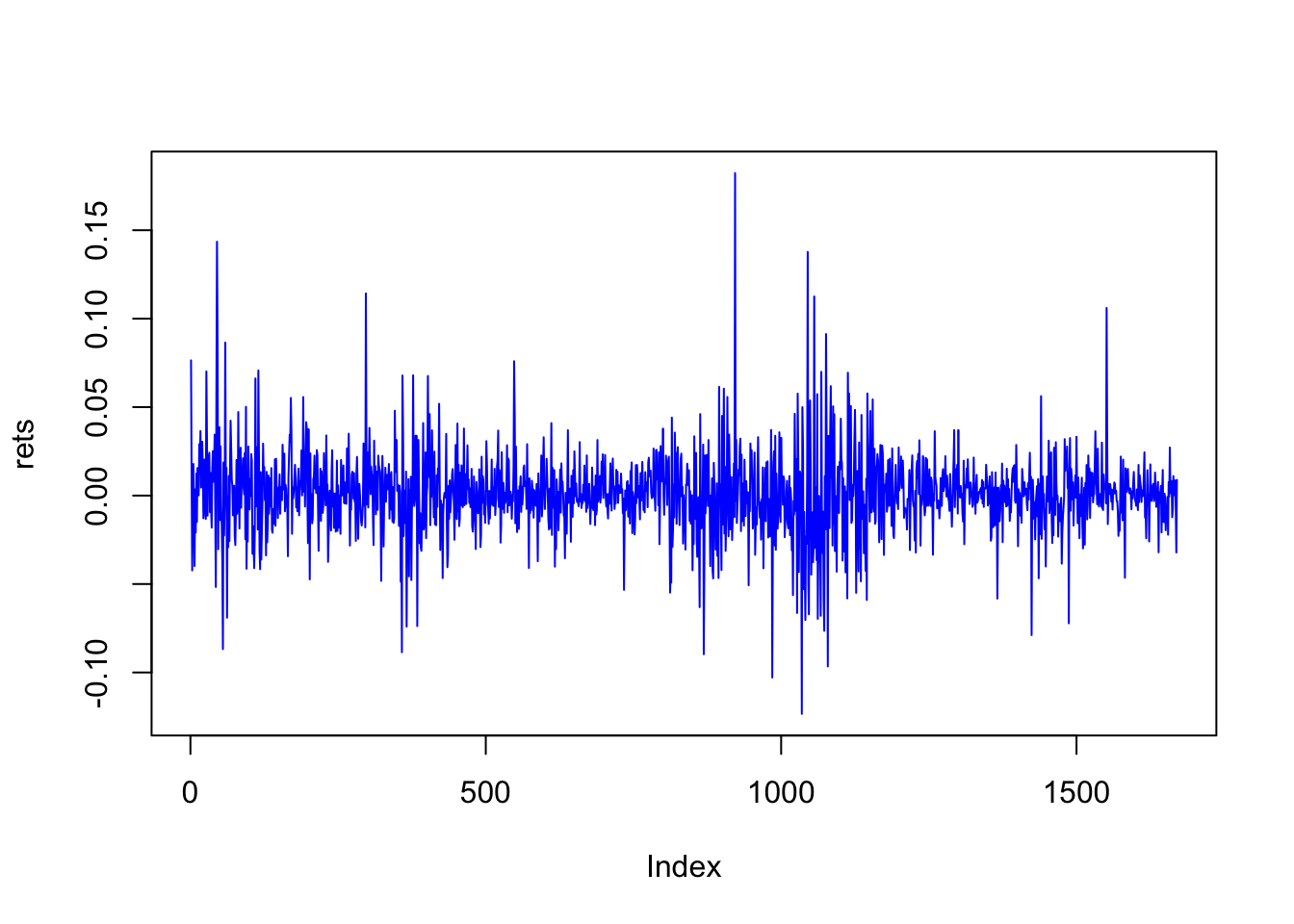
print(n)## [1] 1670Examine the autocorrelation. This is one lag, also known as first-order autocorrelation.
cor(rets[1:(n-1)],rets[2:n])## [1] 0.007215026Run the Durbin-Watson test for autocorrelation. Here we test for up to 10 lags.
library(car)
res = lm(rets[2:n]~rets[1:(n-1)])
durbinWatsonTest(res,max.lag=10)
## lag Autocorrelation D-W Statistic p-value
## 1 -0.0006436855 2.001125 0.950
## 2 -0.0109757002 2.018298 0.696
## 3 -0.0002853870 1.996723 0.982
## 4 0.0252586312 1.945238 0.324
## 5 0.0188824874 1.957564 0.444
## 6 -0.0555810090 2.104550 0.018
## 7 0.0020507562 1.989158 0.986
## 8 0.0746953706 1.843219 0.004
## 9 -0.0375308940 2.067304 0.108
## 10 0.0085641680 1.974756 0.798
## Alternative hypothesis: rho[lag] != 0There is no evidence of auto-correlation when the DW statistic is close to 2. If the DW-statistic is greater than 2 it indicates negative autocorrelation, and if it is less than 2, it indicates positive autocorrelation.
If there is autocorrelation we can correct for it as follows. Let’s take a different data set.
md = read.table("DSTMAA_data/markowitzdata.txt",header=TRUE)
names(md)
## [1] "X.DATE" "SUNW" "MSFT" "IBM" "CSCO" "AMZN" "mktrf"
## [8] "smb" "hml" "rf"Test for autocorrelation.
y = as.matrix(md[2])
x = as.matrix(md[7:9])
rf = as.matrix(md[10])
y = y-rf
library(car)
results = lm(y ~ x)
print(summary(results))
##
## Call:
## lm(formula = y ~ x)
##
## Residuals:
## Min 1Q Median 3Q Max
## -0.213676 -0.014356 -0.000733 0.014462 0.191089
##
## Coefficients:
## Estimate Std. Error t value Pr(>|t|)
## (Intercept) -0.000197 0.000785 -0.251 0.8019
## xmktrf 1.657968 0.085816 19.320 <2e-16 ***
## xsmb 0.299735 0.146973 2.039 0.0416 *
## xhml -1.544633 0.176049 -8.774 <2e-16 ***
## ---
## Signif. codes: 0 '***' 0.001 '**' 0.01 '*' 0.05 '.' 0.1 ' ' 1
##
## Residual standard error: 0.03028 on 1503 degrees of freedom
## Multiple R-squared: 0.3636, Adjusted R-squared: 0.3623
## F-statistic: 286.3 on 3 and 1503 DF, p-value: < 2.2e-16durbinWatsonTest(results,max.lag=6)## lag Autocorrelation D-W Statistic p-value
## 1 -0.07231926 2.144549 0.008
## 2 -0.04595240 2.079356 0.122
## 3 0.02958136 1.926791 0.180
## 4 -0.01608143 2.017980 0.654
## 5 -0.02360625 2.032176 0.474
## 6 -0.01874952 2.021745 0.594
## Alternative hypothesis: rho[lag] != 0Now make the correction to the t-statistics. We use the procedure formulated by Newey and West (1987). This correction is part of the car package.
#CORRECT FOR AUTOCORRELATION
library(sandwich)
b = results$coefficients
print(b)
## (Intercept) xmktrf xsmb xhml
## -0.0001970164 1.6579682191 0.2997353765 -1.5446330690vb = NeweyWest(results,lag=1)
stdb = sqrt(diag(vb))
tstats = b/stdb
print(tstats)## (Intercept) xmktrf xsmb xhml
## -0.2633665 15.5779184 1.8300340 -6.1036120Compare these to the stats we had earlier. Notice how they have come down after correction for AR. Note that there are several steps needed to correct for autocorrelation, and it might have been nice to roll one’s own function for this. (I leave this as an exercise for you.)
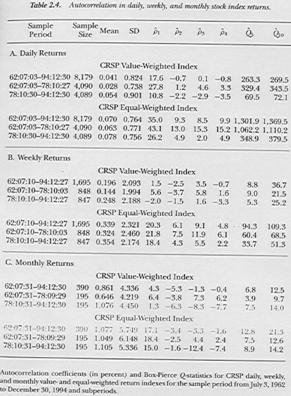
Figure 3.1: From Lo and MacKinlay (1999)
For fun, lets look at the autocorrelation in stock market indexes, shown in Figure 3.1. The following graphic is taken from the book “A Non-Random Walk Down Wall Street” by A. W. Lo and MacKinlay (1999). Is the autocorrelation higher for equally-weighted or value-weighted indexes? Why?
3.14 Maximum Likelihood
Assume that the stock returns \(R(t)\) mentioned above have a normal distribution with mean \(\mu\) and variance \(\sigma^2\) per year. MLE estimation requires finding the parameters \(\{\mu,\sigma\}\) that maximize the likelihood of seeing the empirical sequence of returns \(R(t)\). A normal probability function is required, and we have one above for \(R(t)\), which is assumed to be i.i.d. (independent and identically distributed).
First, a quick recap of the normal distribution. If \(x \sim N(\mu,\sigma^2)\), then \[\begin{equation} \mbox{density function:} \quad f(x) = \frac{1}{\sqrt{2\pi\sigma^2}} \exp\left[-\frac{1}{2}\frac{(x-\mu)^2}{\sigma^2} \right] \end{equation}\] \[\begin{equation} N(x) = 1 - N(-x) \end{equation}\] \[\begin{equation} F(x) = \int_{-\infty}^x f(u) du \end{equation}\]The standard normal distribution is \(x \sim N(0,1)\). For the standard normal distribution: \(F(0) = \frac{1}{2}\).
Noting that when returns are i.i.d., the mean return and the variance of returns scale with time, and therefore, the standard deviation of returns scales with the square-root of time. If the time intervals between return observations is \(h\) years, then the probability density of \(R(t)\) is normal with the following equation:
\[\begin{equation} f[R(t)] = \frac{1}{\sqrt{2 \pi \sigma^2 h}} \cdot \exp\left[ -\frac{1}{2} \cdot \frac{(R(t)-\alpha)^2}{\sigma^2 h} \right] \end{equation}\]where \(\alpha = \left(\mu-\frac{1}{2}\sigma^2 \right) h\). In our case, we have daily data and \(h=1/252\). For periods \(t=1,2,\ldots,T\) the likelihood of the entire series is
\[\begin{equation} \prod_{t=1}^T f[R(t)] \end{equation}\] It is easier (computationally) to maximize \[\begin{equation} \max_{\mu,\sigma} \; {\cal L} \equiv \sum_{t=1}^T \ln f[R(t)] \end{equation}\]known as the log-likelihood. This is easily done in R. First we create the log-likelihood function, so you can see how functions are defined in R.
Note that \[\begin{equation} \ln \; f[R(t)] = -\ln \sqrt{2 \pi \sigma^2 h} - \frac{[R(t)-\alpha]^2}{2 \sigma^2 h} \end{equation}\]We have used variable “sigsq” in function “LL” for \(\sigma^2 h\).
#LOG-LIKELIHOOD FUNCTION
LL = function(params,rets) {
    alpha = params[1]; sigsq = params[2]
    logf = -log(sqrt(2*pi*sigsq)) - (rets-alpha)^2/(2*sigsq)
    LL = -sum(logf)
}
We now read in the data and maximize the log-likelihood to find the required parameters of the return distribution.
#READ DATA
data = read.csv("DSTMAA_data/goog.csv",header=TRUE)
stkp = data$Adj.Close
#Ln of differenced stk prices gives continuous returns
rets = diff(log(stkp))  #diff() takes first differences
print(c("mean return = ",mean(rets),mean(rets)*252))
## [1] "mean return = " "-0.00104453803410475" "-0.263223584594396"print(c("stdev returns = ",sd(rets),sd(rets)*sqrt(252)))## [1] "stdev returns = " "0.0226682330750677" "0.359847044267268"#Create starting guess for parameters
params = c(0.001,0.001)
res = nlm(LL,params,rets)
print(res)## $minimum
## [1] -3954.813
##
## $estimate
## [1] -0.0010450602 0.0005130408
##
## $gradient
## [1] -0.07215158 -1.93982032
##
## $code
## [1] 2
##
## $iterations
## [1] 8Let’s annualize the parameters and see what they are, comparing them to the raw mean and variance of returns.
h = 1/252
alpha = res$estimate[1]
sigsq = res$estimate[2]
print(c("alpha=",alpha))
## [1] "alpha=" "-0.00104506019968994"print(c("sigsq=",sigsq))## [1] "sigsq=" "0.000513040809008682"sigma = sqrt(sigsq/h)
mu = alpha/h + 0.5*sigma^2
print(c("mu=",mu))## [1] "mu=" "-0.19871202838677"print(c("sigma=",sigma))## [1] "sigma=" "0.359564019154014"print(mean(rets*252))## [1] -0.2632236print(sd(rets)*sqrt(252))## [1] 0.359847As we can see, the parameters under the normal distribution are quite close to the raw moments.
3.15 Logit
We have seen how to fit a linear regression model in R. In that model we placed no restrictions on the dependent variable. However, when the LHS variable in a regression is categorical and binary, i.e., takes the value 1 or 0, then a logit regression is more apt. This regression fits a model that will always return a fitted value of the dependent variable that lies between \((0,1)\). This class of specifications covers what are known as limited dependent variables models. In this introduction to R, we will simply run a few examples of these models, leaving a more detailed analysis for later in this book.
Example: For the NCAA data, there are 64 observatios (teams) ordered from best to worst. We take the top 32 teams and make their dependent variable 1 (above median teams), and that of the bottom 32 teams zero (below median). Our goal is to fit a regression model that returns a team’s predicted percentile ranking.
First, we create the dependent variable.
y = c(rep(1,32),rep(0,32))
print(y)
## [1] 1 1 1 1 1 1 1 1 1 1 1 1 1 1 1 1 1 1 1 1 1 1 1 1 1 1 1 1 1 1 1 1 0 0 0
## [36] 0 0 0 0 0 0 0 0 0 0 0 0 0 0 0 0 0 0 0 0 0 0 0 0 0 0 0 0 0x = as.matrix(ncaa[,4:14])
y = as.matrix(y)We use the function glm for this task. Running the model is pretty easy as follows.
h = glm(y~x, family=binomial(link="logit"))
print(logLik(h))
## 'log Lik.' -21.44779 (df=12)print(summary(h))##
## Call:
## glm(formula = y ~ x, family = binomial(link = "logit"))
##
## Deviance Residuals:
## Min 1Q Median 3Q Max
## -1.80174 -0.40502 -0.00238 0.37584 2.31767
##
## Coefficients:
## Estimate Std. Error z value Pr(>|z|)
## (Intercept) -45.83315 14.97564 -3.061 0.00221 **
## xPTS -0.06127 0.09549 -0.642 0.52108
## xREB 0.49037 0.18089 2.711 0.00671 **
## xAST 0.16422 0.26804 0.613 0.54010
## xTO -0.38405 0.23434 -1.639 0.10124
## xA.T 1.56351 3.17091 0.493 0.62196
## xSTL 0.78360 0.32605 2.403 0.01625 *
## xBLK 0.07867 0.23482 0.335 0.73761
## xPF 0.02602 0.13644 0.191 0.84874
## xFG 46.21374 17.33685 2.666 0.00768 **
## xFT 10.72992 4.47729 2.397 0.01655 *
## xX3P 5.41985 5.77966 0.938 0.34838
## ---
## Signif. codes: 0 '***' 0.001 '**' 0.01 '*' 0.05 '.' 0.1 ' ' 1
##
## (Dispersion parameter for binomial family taken to be 1)
##
## Null deviance: 88.723 on 63 degrees of freedom
## Residual deviance: 42.896 on 52 degrees of freedom
## AIC: 66.896
##
## Number of Fisher Scoring iterations: 6Thus, we see that the best variables that separate upper-half teams from lower-half teams are the number of rebounds and the field goal percentage. To a lesser extent, field goal percentage and steals also provide some explanatory power. The logit regression is specified as follows:
\[\begin{eqnarray*} z &=& \frac{e^y}{1+e^y}\\ y &=& b_0 + b_1 x_1 + b_2 x_2 + \ldots + b_k x_k \end{eqnarray*}\]The original data \(z = \{0,1\}\). The range of values of \(y\) is \((-\infty,+\infty)\). And as required, the fitted \(z \in (0,1)\). The variables \(x\) are the RHS variables. The fitting is done using MLE.
Suppose we ran this with a simple linear regression.
h = lm(y~x)
summary(h)
##
## Call:
## lm(formula = y ~ x)
##
## Residuals:
## Min 1Q Median 3Q Max
## -0.65982 -0.26830 0.03183 0.24712 0.83049
##
## Coefficients:
## Estimate Std. Error t value Pr(>|t|)
## (Intercept) -4.114185 1.174308 -3.503 0.000953 ***
## xPTS -0.005569 0.010263 -0.543 0.589709
## xREB 0.046922 0.015003 3.128 0.002886 **
## xAST 0.015391 0.036990 0.416 0.679055
## xTO -0.046479 0.028988 -1.603 0.114905
## xA.T 0.103216 0.450763 0.229 0.819782
## xSTL 0.063309 0.028015 2.260 0.028050 *
## xBLK 0.023088 0.030474 0.758 0.452082
## xPF 0.011492 0.018056 0.636 0.527253
## xFG 4.842722 1.616465 2.996 0.004186 **
## xFT 1.162177 0.454178 2.559 0.013452 *
## xX3P 0.476283 0.712184 0.669 0.506604
## ---
## Signif. codes: 0 '***' 0.001 '**' 0.01 '*' 0.05 '.' 0.1 ' ' 1
##
## Residual standard error: 0.3905 on 52 degrees of freedom
## Multiple R-squared: 0.5043, Adjusted R-squared: 0.3995
## F-statistic: 4.81 on 11 and 52 DF, p-value: 4.514e-05We get the same variables again showing up as significant.
3.16 Probit
We can redo the same regression in the logit using a probit instead. A probit is identical in spirit to the logit regression, except that the function that is used is
\[\begin{eqnarray*} z &=& \Phi(y)\\ y &=& b_0 + b_1 x_1 + b_2 x_2 + \ldots + b_k x_k \end{eqnarray*}\]where \(\Phi(\cdot)\) is the cumulative normal probability function. It is implemented in R as follows.
h = glm(y~x, family=binomial(link="probit"))
print(logLik(h))
## 'log Lik.' -21.27924 (df=12)print(summary(h))##
## Call:
## glm(formula = y ~ x, family = binomial(link = "probit"))
##
## Deviance Residuals:
## Min 1Q Median 3Q Max
## -1.76353 -0.41212 -0.00031 0.34996 2.24568
##
## Coefficients:
## Estimate Std. Error z value Pr(>|z|)
## (Intercept) -26.28219 8.09608 -3.246 0.00117 **
## xPTS -0.03463 0.05385 -0.643 0.52020
## xREB 0.28493 0.09939 2.867 0.00415 **
## xAST 0.10894 0.15735 0.692 0.48874
## xTO -0.23742 0.13642 -1.740 0.08180 .
## xA.T 0.71485 1.86701 0.383 0.70181
## xSTL 0.45963 0.18414 2.496 0.01256 *
## xBLK 0.03029 0.13631 0.222 0.82415
## xPF 0.01041 0.07907 0.132 0.89529
## xFG 26.58461 9.38711 2.832 0.00463 **
## xFT 6.28278 2.51452 2.499 0.01247 *
## xX3P 3.15824 3.37841 0.935 0.34988
## ---
## Signif. codes: 0 '***' 0.001 '**' 0.01 '*' 0.05 '.' 0.1 ' ' 1
##
## (Dispersion parameter for binomial family taken to be 1)
##
## Null deviance: 88.723 on 63 degrees of freedom
## Residual deviance: 42.558 on 52 degrees of freedom
## AIC: 66.558
##
## Number of Fisher Scoring iterations: 8The results confirm those obtained from the linear regression and logit regression.
3.17 ARCH and GARCH
GARCH stands for “Generalized Auto-Regressive Conditional Heteroskedasticity”. Engle (1982) invented ARCH (for which he got the Nobel prize) and this was extended by Bollerslev (1986) to GARCH.
ARCH models are based on the idea that volatility tends to cluster, i.e., volatility for period \(t\), is auto-correlated with volatility from period \((t-1)\), or more preceding periods. If we had a time series of stock returns following a random walk, we might model it as follows
\[\begin{equation} r_t = \mu + e_t, \quad e_t \sim N(0,\sigma_t^2) \end{equation}\]Returns have constant mean \(\mu\) and time-varying variance \(\sigma_t^2\). If the variance were stationary then \(\sigma_t^2\) would be constant. But under GARCH it is auto-correlated with previous variances. Hence, we have
\[\begin{equation} \sigma_{t}^2 = \beta_0 + \sum_{j=1}^p \beta_{1j} \sigma_{t-j}^2 + \sum_{k=1}^q \beta_{2k} e_{t-k}^2 \end{equation}\]So current variance (\(\sigma_t^2\)) depends on past squared shocks (\(e_{t-k}^2\)) and past variances (\(\sigma_{t-j}^2\)). The number of lags of past variance is \(p\), and that of lagged shocks is \(q\). The model is thus known as a GARCH\((p,q)\) model. For the model to be stationary, the sum of all the \(\beta\) terms should be less than 1.
In GARCH, stock returns are conditionally normal, and independent, but not identically distributed because the variance changes over time. Since at every time \(t\), we know the conditional distribution of returns, because \(\sigma_t\) is based on past \(\sigma_{t-j}\) and past shocks \(e_{t-k}\), we can estimate the parameters \(\{\beta_0,\beta{1j}, \beta_{2k}\}, \forall j,k\), of the model using MLE. The good news is that this comes canned in R, so all we need to do is use the tseries package.
library(tseries)
res = garch(rets,order=c(1,1))
##
## ***** ESTIMATION WITH ANALYTICAL GRADIENT *****
##
##
## I INITIAL X(I) D(I)
##
## 1 4.624639e-04 1.000e+00
## 2 5.000000e-02 1.000e+00
## 3 5.000000e-02 1.000e+00
##
## IT NF F RELDF PRELDF RELDX STPPAR D*STEP NPRELDF
## 0 1 -5.512e+03
## 1 7 -5.513e+03 1.82e-04 2.97e-04 2.0e-04 4.3e+09 2.0e-05 6.33e+05
## 2 8 -5.513e+03 8.45e-06 9.19e-06 1.9e-04 2.0e+00 2.0e-05 1.57e+01
## 3 15 -5.536e+03 3.99e-03 6.04e-03 4.4e-01 2.0e+00 8.0e-02 1.56e+01
## 4 18 -5.569e+03 6.02e-03 4.17e-03 7.4e-01 1.9e+00 3.2e-01 4.54e-01
## 5 20 -5.579e+03 1.85e-03 1.71e-03 7.9e-02 2.0e+00 6.4e-02 1.67e+02
## 6 22 -5.604e+03 4.44e-03 3.94e-03 1.3e-01 2.0e+00 1.3e-01 1.93e+04
## 7 24 -5.610e+03 9.79e-04 9.71e-04 2.2e-02 2.0e+00 2.6e-02 2.93e+06
## 8 26 -5.621e+03 1.92e-03 1.96e-03 4.1e-02 2.0e+00 5.1e-02 2.76e+08
## 9 27 -5.639e+03 3.20e-03 4.34e-03 7.4e-02 2.0e+00 1.0e-01 2.26e+02
## 10 34 -5.640e+03 2.02e-04 3.91e-04 3.7e-06 4.0e+00 5.5e-06 1.73e+01
## 11 35 -5.640e+03 7.02e-06 8.09e-06 3.6e-06 2.0e+00 5.5e-06 5.02e+00
## 12 36 -5.640e+03 2.22e-07 2.36e-07 3.7e-06 2.0e+00 5.5e-06 5.26e+00
## 13 43 -5.641e+03 2.52e-04 3.98e-04 1.5e-02 2.0e+00 2.3e-02 5.26e+00
## 14 45 -5.642e+03 2.28e-04 1.40e-04 1.7e-02 0.0e+00 3.2e-02 1.40e-04
## 15 46 -5.644e+03 3.17e-04 3.54e-04 3.9e-02 1.0e-01 8.8e-02 3.57e-04
## 16 56 -5.644e+03 1.60e-05 3.69e-05 5.7e-07 3.2e+00 9.7e-07 6.48e-05
## 17 57 -5.644e+03 1.91e-06 1.96e-06 5.0e-07 2.0e+00 9.7e-07 1.20e-05
## 18 58 -5.644e+03 8.57e-11 5.45e-09 5.2e-07 2.0e+00 9.7e-07 9.38e-06
## 19 66 -5.644e+03 6.92e-06 9.36e-06 4.2e-03 6.2e-02 7.8e-03 9.38e-06
## 20 67 -5.644e+03 7.42e-07 1.16e-06 1.2e-03 0.0e+00 2.2e-03 1.16e-06
## 21 68 -5.644e+03 8.44e-08 1.50e-07 7.1e-04 0.0e+00 1.6e-03 1.50e-07
## 22 69 -5.644e+03 1.39e-08 2.44e-09 8.6e-05 0.0e+00 1.8e-04 2.44e-09
## 23 70 -5.644e+03 -7.35e-10 1.24e-11 3.1e-06 0.0e+00 5.4e-06 1.24e-11
##
## ***** RELATIVE FUNCTION CONVERGENCE *****
##
## FUNCTION -5.644379e+03 RELDX 3.128e-06
## FUNC. EVALS 70 GRAD. EVALS 23
## PRELDF 1.242e-11 NPRELDF 1.242e-11
##
## I FINAL X(I) D(I) G(I)
##
## 1 1.807617e-05 1.000e+00 1.035e+01
## 2 1.304314e-01 1.000e+00 -2.837e-02
## 3 8.457819e-01 1.000e+00 -2.915e-02summary(res)##
## Call:
## garch(x = rets, order = c(1, 1))
##
## Model:
## GARCH(1,1)
##
## Residuals:
## Min 1Q Median 3Q Max
## -9.17102 -0.59191 -0.03853 0.43929 4.64677
##
## Coefficient(s):
## Estimate Std. Error t value Pr(>|t|)
## a0 1.808e-05 2.394e-06 7.551 4.33e-14 ***
## a1 1.304e-01 1.292e-02 10.094 < 2e-16 ***
## b1 8.458e-01 1.307e-02 64.720 < 2e-16 ***
## ---
## Signif. codes: 0 '***' 0.001 '**' 0.01 '*' 0.05 '.' 0.1 ' ' 1
##
## Diagnostic Tests:
## Jarque Bera Test
##
## data: Residuals
## X-squared = 3199.7, df = 2, p-value < 2.2e-16
##
##
## Box-Ljung test
##
## data: Squared.Residuals
## X-squared = 0.14094, df = 1, p-value = 0.7073That’s it! Certainly much less painful than programming the entire MLE procedure. We see that the parameters \(\{\beta_0,\beta_1,\beta_2\}\) are all statistically significant. Given the fitted parameters, we can also examine the extracted time series of volatilty.
#PLOT VOLATILITY TIMES SERIES
print(names(res))
## [1] "order" "coef" "n.likeli" "n.used"
## [5] "residuals" "fitted.values" "series" "frequency"
## [9] "call" "vcov"plot(res$fitted.values[,1],type="l",col="red")
grid(lwd=2)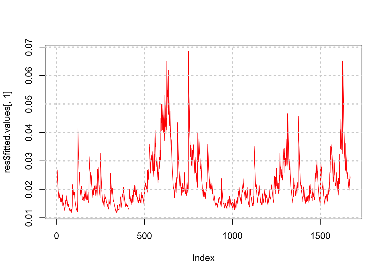
We may also plot is side by side with the stock price series.
par(mfrow=c(2,1))
plot(res$fitted.values[,1],col="blue",type="l")
plot(stkp,type="l",col="red")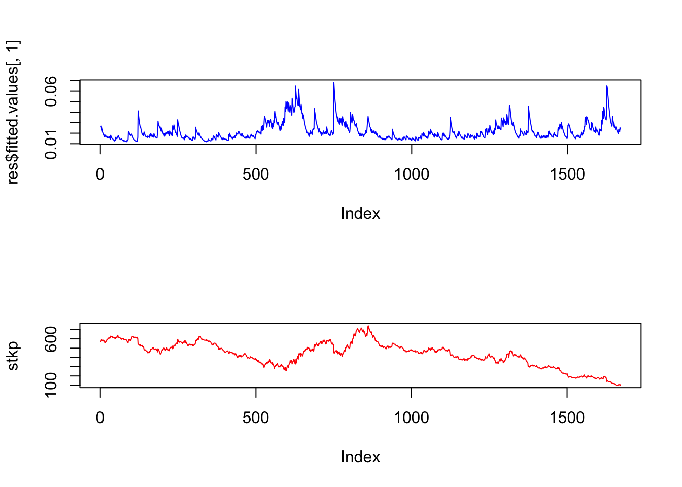
Notice how the volatility series clumps into periods of high volatility, interspersed with larger periods of calm. As is often the case, volatility tends to be higher when the stock price is lower.
3.18 Vector Autoregression
Also known as VAR (not the same thing as Value-at-Risk, denoted VaR). VAR is useful for estimating systems where there are simultaneous regression equations, and the variables influence each other over time. So in a VAR, each variable in a system is assumed to depend on lagged values of itself and the other variables. The number of lags may be chosen by the econometrician based on the expected decay in time-dependence of the variables in the VAR.
In the following example, we examine the inter-relatedness of returns of the following three tickers: SUNW, MSFT, IBM. For vector autoregressions (VARs), we run the following R commands:
md = read.table("DSTMAA_data/markowitzdata.txt",header=TRUE)
y = as.matrix(md[2:4])
library(stats)
var6 = ar(y,aic=TRUE,order=6)
print(var6$order)
## [1] 1print(var6$ar)## , , SUNW
##
## SUNW MSFT IBM
## 1 -0.00985635 0.02224093 0.002072782
##
## , , MSFT
##
## SUNW MSFT IBM
## 1 0.008658304 -0.1369503 0.0306552
##
## , , IBM
##
## SUNW MSFT IBM
## 1 -0.04517035 0.0975497 -0.01283037We print out the Akaike Information Criterion (AIC)28 to see which lags are significant.
print(var6$aic)## 0 1 2 3 4 5 6
## 23.950676 0.000000 2.762663 5.284709 5.164238 10.065300 8.924513Since there are three stocks’ returns moving over time, we have a system of three equations, each with six lags, so there will be six lagged coefficients for each equation. We print out these coefficients here, and examine the sign. We note however that only one lag is significant, as the “order” of the system was estimated as 1 in the VAR above.
print(var6$partialacf)## , , SUNW
##
## SUNW MSFT IBM
## 1 -0.00985635 0.022240931 0.002072782
## 2 -0.07857841 -0.019721982 -0.006210487
## 3 0.03382375 0.003658121 0.032990758
## 4 0.02259522 0.030023132 0.020925226
## 5 -0.03944162 -0.030654949 -0.012384084
## 6 -0.03109748 -0.021612632 -0.003164879
##
## , , MSFT
##
## SUNW MSFT IBM
## 1 0.008658304 -0.13695027 0.030655201
## 2 -0.053224374 -0.02396291 -0.047058278
## 3 0.080632420 0.03720952 -0.004353203
## 4 -0.038171317 -0.07573402 -0.004913021
## 5 0.002727220 0.05886752 0.050568308
## 6 0.242148823 0.03534206 0.062799122
##
## , , IBM
##
## SUNW MSFT IBM
## 1 -0.04517035 0.097549700 -0.01283037
## 2 0.05436993 0.021189756 0.05430338
## 3 -0.08990973 -0.077140955 -0.03979962
## 4 0.06651063 0.056250866 0.05200459
## 5 0.03117548 -0.056192843 -0.06080490
## 6 -0.13131366 -0.003776726 -0.01502191Interestingly we see that each of the tickers has a negative relation to its lagged value, but a positive correlation with the lagged values of the other two stocks. Hence, there is positive cross autocorrelation amongst these tech stocks. We can also run a model with three lags.
ar(y,method="ols",order=3)##
## Call:
## ar(x = y, order.max = 3, method = "ols")
##
## $ar
## , , 1
##
## SUNW MSFT IBM
## SUNW 0.01407 -0.0006952 -0.036839
## MSFT 0.02693 -0.1440645 0.100557
## IBM 0.01330 0.0211160 -0.009662
##
## , , 2
##
## SUNW MSFT IBM
## SUNW -0.082017 -0.04079 0.04812
## MSFT -0.020668 -0.01722 0.01761
## IBM -0.006717 -0.04790 0.05537
##
## , , 3
##
## SUNW MSFT IBM
## SUNW 0.035412 0.081961 -0.09139
## MSFT 0.003999 0.037252 -0.07719
## IBM 0.033571 -0.003906 -0.04031
##
##
## $x.intercept
## SUNW MSFT IBM
## -9.623e-05 -7.366e-05 -6.257e-05
##
## $var.pred
## SUNW MSFT IBM
## SUNW 0.0013593 0.0003007 0.0002842
## MSFT 0.0003007 0.0003511 0.0001888
## IBM 0.0002842 0.0001888 0.0002881We examine cross autocorrelation found across all stocks by Lo and Mackinlay in their book “A Non-Random Walk Down Wall Street” – see Figure 3.2.
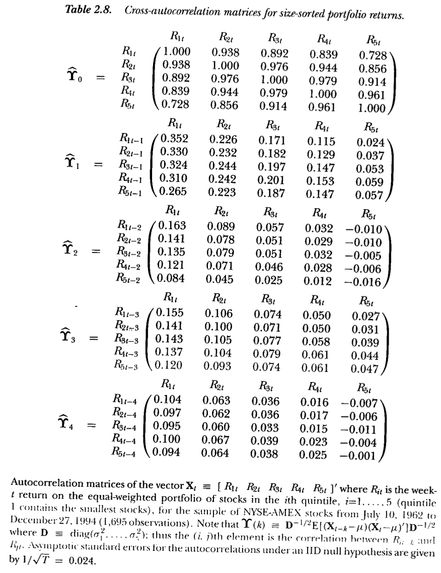
Figure 3.2: From Lo and MacKinlay (1999)
We see that one-lag cross autocorrelations are positive. Compare these portfolio autocorrelations with the individual stock autocorrelations in the example here.
3.19 Solving Non-Linear Equations
Earlier we examined root finding. Here we develop it further. We have also not done much with user-generated functions. Here is a neat model in R to solve for the implied volatility in the Black-Merton-Scholes class of models. First, we code up the Black and Scholes (1973) model; this is the function bms73 below. Then we write a user-defined function that solves for the implied volatility from a given call or put option price. The package minpack.lm is used for the equation solving, and the function call is nls.lm.
If you are not familiar with the Nobel Prize winning Black-Scholes model, never mind, almost the entire world has never heard of it. Just think of it as a nonlinear multivariate function that we will use as an exemplar for equation solving. We are going to use the function below to solve for the value of sig in the expressions below. We set up two functions.
#Black-Merton-Scholes 1973
#sig: volatility
#S: stock price
#K: strike price
#T: maturity
#r: risk free rate
#q: dividend rate
#cp = 1 for calls and -1 for puts
#optprice: observed option price
bms73 = function(sig,S,K,T,r,q,cp=1,optprice) {
    d1 = (log(S/K)+(r-q+0.5*sig^2)*T)/(sig*sqrt(T))
    d2 = d1 - sig*sqrt(T)
    if (cp==1) {
        optval = S*exp(-q*T)*pnorm(d1)-K*exp(-r*T)*pnorm(d2)
        }
    else {
        optval = -S*exp(-q*T)*pnorm(-d1)+K*exp(-r*T)*pnorm(-d2)
    }
    #If option price is supplied we want the implied vol, else optprice
    bs = optval - optprice
}

#Function to return Imp Vol with starting guess sig0
impvol = function(sig0,S,K,T,r,q,cp,optprice) {
    sol = nls.lm(par=sig0,fn=bms73,S=S,K=K,T=T,r=r,q=q,
          cp=cp,optprice=optprice)
}
We use the minimizer to solve the nonlinear function for the value of sig. The calls to this model are as follows:
library(minpack.lm)
optprice = 4
res = impvol(0.2,40,40,1,0.03,0,-1,optprice)
print(names(res))
## [1] "par" "hessian" "fvec" "info" "message" "diag"
## [7] "niter" "rsstrace" "deviance"print(c("Implied vol = ",res$par))## [1] "Implied vol = " "0.291522285803426"We note that the function impvol was written such that the argument that we needed to solve for, sig0, the implied volatility, was the first argument in the function. However, the expression par=sig0 does inform the solver which argument is being searched for in order to satisfy the non-linear equation for implied volatility. Note also that the function bms73 returns the difference between the model price and observed price, not the model price alone. This is necessary as the solver tries to set this function value to zero by finding the implied volatility.
Lets check if we put this volatility back into the bms function that we get back the option price of 4. Voila!
#CHECK
optp = bms73(res$par,40,40,1,0.03,0,0,4) + optprice
print(c("Check option price = ",optp))
## [1] "Check option price = " "4"3.20 Web-Enabling R Functions
We may be interested in hosting our R programs for users to run through a browser interface. This section walks you through the process to do so. This is an extract of my blog post at http://sanjivdas.wordpress.com/2010/11/07/web-enabling-r-functions-with-cgi-on-a-mac-os-x-desktop/. The same may be achieved by using the Shiny package in R, which enables you to create interactive browser-based applications, and is in fact a more powerful environment in which to create web-driven applications. See: https://shiny.rstudio.com/.
Here we desribe an example based on the Rcgi package from David Firth, and for full details of using R with CGI, see http://www.omegahat.org/CGIwithR/. Download the document on using R with CGI. It’s titled “CGIwithR: Facilities for Processing Web Forms with R.”29
You need two program files to get everything working. (These instructions are for a Mac environment.)
- The html file that is the web form for input data.
- The R file, with special tags for use with the CGIwithR package.
Our example will be simple, i.e., a calculator to work out the monthly payment on a standard fixed rate mortgage. The three inputs are the loan principal, annual loan rate, and the number of remaining months to maturity.
But first, let’s create the html file for the web page that will take these three input values. We call it mortgage_calc.html. The code is all standard, for those familiar with html, and even if you are not used to html, the code is self-explanatory. See Figure 3.3.
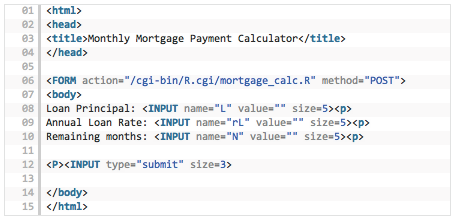
Figure 3.3: HTML code for the Rcgi application
Notice that line 06 will be the one referencing the R program that does the calculation. The three inputs are accepted in lines 08-10. Line 12 sends the inputs to the R program.
Next, we look at the R program, suitably modified to include html tags. We name it mortgage_calc.R. See Figure 3.4.
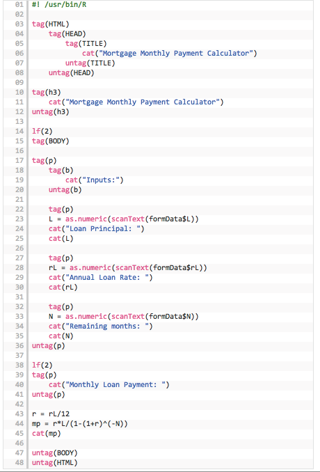
Figure 3.4: R code for the Rcgi application
We can see that all html calls in the R program are made using the tag() construct. Lines 22–35 take in the three inputs from the html form. Lines 43–44 do the calculations and line 45 prints the result. The cat() function prints its arguments to the web browser page.
Okay, we have seen how the two programs (html, R) are written and these templates may be used with changes as needed. We also need to pay attention to setting up the R environment to make sure that the function is served up by the system. The following steps are needed:
Make sure that your Mac is allowing connections to its web server. Go to System Preferences and choose Sharing. In this window enable Web Sharing by ticking the box next to it.
Place the html file mortgage_calc.html in the directory that serves up web pages. On a Mac, there is already a web directory for this called Sites. It’s a good idea to open a separate subdirectory called (say) Rcgi below this one for the R related programs and put the html file there.
The R program mortgage_calc.R must go in the directory that has been assigned for CGI executables. On a Mac, the default for this directory is /Library/WebServer/CGI-Executables and is usually referenced by the alias cgi-bin (stands for cgi binaries). Drop the R program into this directory.
Two more important files are created when you install the Rcgi package. The CGIwithR installation creates two files:
- A hidden file called .Rprofile;
- A file called R.cgi.
Place both these files in the directory: /Library/WebServer/CGI-Executables.
If you cannot find the .Rprofile file then create it directly by opening a text editor and adding two lines to the file:
#! /usr/bin/R
library(CGIwithR,warn.conflicts=FALSE)
Now, open the R.cgi file and make sure that the line pointing to the R executable in the file is showing
R_DEFAULT=/usr/bin/R
The file may actually have it as #!/usr/local/bin/R which is for Linux platforms, but the usual Mac install has the executable in #! /usr/bin/R so make sure this is done.
Make both files executable as follows: > chmod a+rx .Rprofile > chmod a+rx R.cgi
Finally, make the \(\sim\)/Sites/Rcgi/ directory write accessible:
chmod a+wx \(\sim\)/Sites/Rcgi
Just being patient and following all the steps makes sure it all works well. Having done it once, it’s easy to repeat and create several functions. The inputs are as follows: Loan principal (enter a dollar amount). Annual loan rate (enter it in decimals, e.g., six percent is entered as 0.06). Remaining maturity in months (enter 300 if the remaining maturity is 25 years).
References
Newey, Whitney K., and Kenneth D. West. 1987. “A Simple, Positive Semi-Definite, Heteroskedasticity and Autocorrelation Consistent Covariance Matrix.” Econometrica 55 (3). [Wiley, Econometric Society]: 703–8. http://www.jstor.org/stable/1913610.
Lo, Andrew W., and A. Craig MacKinlay. 1999. A Non-Random Walk down Wall Street. Princeton University Press. http://www.jstor.org/stable/j.ctt7tccx.
Engle, Robert F. 1982. “Autoregressive Conditional Heteroscedasticity with Estimates of the Variance of United Kingdom Inflation.” Econometrica 50 (4). [Wiley, Econometric Society]: 987–1007. http://www.jstor.org/stable/1912773.
Bollerslev, Tim. 1986. “Generalized autoregressive conditional heteroskedasticity.” Journal of Econometrics 31 (3): 307–27. https://ideas.repec.org/a/eee/econom/v31y1986i3p307-327.html.
Black, Fischer, and Myron Scholes. 1973. “The Pricing of Options and Corporate Liabilities.” Journal of Political Economy 81 (3): 637–54. doi:10.1086/260062.