Chapter 20 Against the Odds: The Mathematics of Gambling

20.1 Introduction

Most people hate mathematics but love gambling. Which of course, is strange because gambling is driven mostly by math. Think of any type of gambling and no doubt there will be maths involved: Horse-track betting, sports betting, blackjack, poker, roulette, stocks, etc.

20.2 Odds

Oddly, bets are defined by their odds. If a bet on a horse is quoted at 4-to-1 odds, it means that if you win, you receive 4 times your wager plus the amount wagered. That is, if you bet $1, you get back $5.

The odds effectively define the probability of winning. Lets define this to be $p$. If the odds are fair, then the expected gain is zero, i.e.

\[ 4p + (1 − p)(−1) = 0 \]

which implies that $p = 1/5$. Hence, if the odds are $x : 1$, then the probability of winning is $p = \frac{1}{x+1} = 0.2$

20.3 Edge

Everyone bets because they think they have an advantage, or an edge over the others. It might be that they just think they have better information, better understanding, are using secret technology, or actually have private information (which may be illegal).

The edge is the expected profit that will be made from repeated trials relative to the bet size. You have an edge if you can win with higher probability ($p^∗$) than $p = 1/(x + 1)$. In the above example, with bet size $1 each time, suppose your probability of winning is not $1/5$, but instead it is $1/4$. What is your edge?

The expected profit is

\[ (−1)×(3/4)+4×(1/4) = 1/4 \]

Dividing this by the bet size (i.e. $1) gives the edge equal to $1/4$.

20.4 Bookmakers

These folks set the odds. Odds are dynamic of course. If the bookie thinks the probability of a win is $1/5$, then he will set the odds to be a bit less than 4:1, maybe something like 3.5:1. In this way his expected intake minus payout is positive. At 3.5:1 odds, if there are still a lot of takers, then the bookie surely realizes that the probability of a win must be higher than in his own estimation. He also infers that $p > 1/(3.5+1)$, and will then change the odds to say 3:1. Therefore, he acts as a market maker in the bet.

20.5 The Kelly Criterion

Suppose you have an edge. How should you bet over repeated plays of the game to maximize your wealth? (Do you think this is the way that hedge funds operate?) The Kelly (1956) criterion says that you should invest only a fraction of your wealth in the bet. By keeping some aside you are guaranteed to not end up in ruin.

What fraction should you bet? The answer is that you should bet

\[ \begin{equation} f = \frac{Edge}{Odds} = \frac{p^∗ x−(1−p^∗)}{x} \end{equation} \]

where the odds are expressed in the form $x : 1$. Recall that $p^∗$ is your privately known probability of winning.

#EXAMPLE
x=4; pstar=1/4; 
f = (pstar*x-(1-pstar))/x
print(c("Kelly share = ",f))

## [1] "Kelly share = " "0.0625"

This means we invest 6.25% of the current bankroll.

20.6 Simulation of the betting strategy

Lets simulate this strategy using R. Here is a simple program to simulate it, with optimal Kelly betting, and over- and under-betting.

#Simulation of the Kelly Criterion

#Basic data
p = 0.25    #private prob of winning
odds = 4    #actual odds
edge = p*odds - (1-p)
f = edge/odds
print(c("edge",edge,"f",f))

## [1] "edge"   "0.25"   "f"      "0.0625"

n = 1000
x = runif(n)
f_over = 1.5*f
f_under = 0.5*f
bankroll = rep(0,n); bankroll[1]=1
br_overbet = bankroll; br_overbet[1]=1
br_underbet = bankroll; br_underbet[1]=1

for (i in 2:n) {
    if (x[i]<=0.25) {
        bankroll[i] = bankroll[i-1] + bankroll[i-1]*f*odds
        br_overbet[i] = br_overbet[i-1] + br_overbet[i-1]*f_over*odds
        br_underbet[i] = br_underbet[i-1] + br_underbet[i-1]*f_under*odds
        }
    else {
        bankroll[i] = bankroll[i-1] - bankroll[i-1]*f
        br_overbet[i] = br_overbet[i-1] - br_overbet[i-1]*f_over
        br_underbet[i] = br_underbet[i-1] - br_underbet[i-1]*f_under
        }
    }

par(mfrow=c(3,1))
plot(bankroll,type="l")
plot(br_overbet,type="l")
plot(br_underbet,type="l")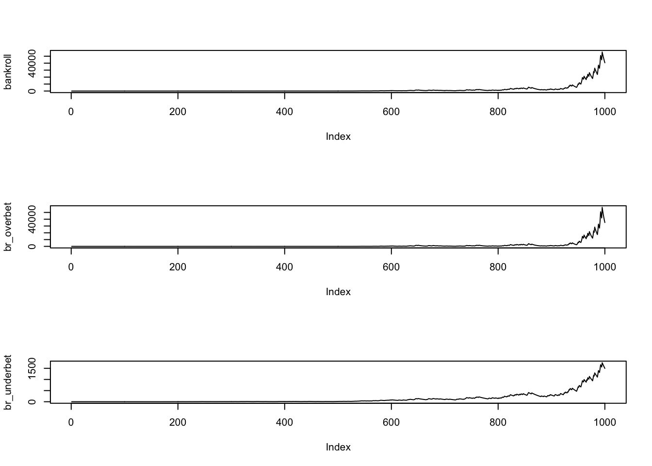

print(c(bankroll[n] ,br_overbet[n] ,br_underbet[n]))

## [1] 40580.312 35159.498  1496.423

print(c(bankroll[n]/br_overbet[n],bankroll[n]/br_underbet[n]))

## [1]  1.154178 27.118207

We repeat this bet a thousand times. The initial pot is $1 only, but after a thousand trials, the optimal strategy ends up being a multiple of the suboptimal ones.

20.7 Half-Kelly

Note here that over-betting is usually worse then under-betting the Kelly optimal. Hence, many players employ what is known as the Half-Kelly rule, i.e., they bet $f/2$.

Look at the resultant plot of the three strategies for the above example. The top plot follows the Kelly criterion, but the other two deviate from it, by overbetting or underbetting the fraction given by Kelly.

We can very clearly see that not betting Kelly leads to far worse outcomes than sticking with the Kelly optimal plan. We ran this for 1000 periods, as if we went to the casino every day and placed one bet (or we placed four bets every minute for about four hours straight). Even within a few trials, the performance of the Kelly is remarkable. Note though that this is only one of the simulated outcomes. The simulations would result in different types of paths of the bankroll value, but generally, the outcomes are similar to what we see in the figure.

Over-betting leads to losses faster than under-betting as one would naturally expect, because it is the more risky strategy.

In this model, under the optimal rule, the probability of dropping to $1/n$ of the bankroll is $1/n$. So the probability of dropping to 90% of the bankroll ($n=1.11$) is $0.9$. Or, there is a 90% chance of losing 10% of the bankroll.

Alternate betting rules are: (a) fixed size bets, (b) double up bets. The former is too slow, the latter ruins eventually.

20.8 Deriving the Kelly Criterion

First we define some notation. Let $B_t$ be the bankroll at time $t$. We index time as going from time $t=1, \ldots, N$.

The odds are denoted, as before $x:1$, and the random variable denoting the outcome (i.e., gains) of the wager is written as

\[ \begin{equation} Z_t = \left\{ \begin{array}{ll} x & \mbox{ w/p } p \\ -1 & \mbox{ w/p } (1-p) \end{array} \right. \end{equation} \]

We are said to have an edge when $E(Z_t)>0$. The edge will be equal to $px-(1-p)>0$.

We invest fraction $f$ of our bankroll, where $0<f<1$, and since $f \neq 1$, there is no chance of being wiped out. Each wager is for an amount $f B_t$ and returns $f B_t Z_t$. Hence, we may write

\[ \begin{eqnarray} B_t &=& B_{t-1} + f B_{t-1} Z_t \\ &=& B_{t-1} [1 + f Z_t] \\ &=& B_0 \prod_{i=1}^t [1+f Z_t] \end{eqnarray} \]

If we define the growth rate as

\[ \begin{eqnarray} g_t(f) &=& \frac{1}{t} \ln \left( \frac{B_t}{B_0} \right) \\ &=& \frac{1}{t} \ln \prod_{i=1}^t [1+f Z_t] \\ &=& \frac{1}{t} \sum_{i=1}^t \ln [1+f Z_t] \end{eqnarray} \]

Taking the limit by applying the law of large numbers, we get

\[ \begin{equation} g(f) = \lim_{t \rightarrow \infty} g_t(f) = E[\ln(1+f Z)] \end{equation} \] which is nothing but the time average of $\ln(1+fZ)$.

We need to find the $f$ that maximizes $g(f)$. We can write this more explicitly as $4 \[ \begin{equation} g(f) = p \ln(1+f x) + (1-p) \ln(1-f) \end{equation} \] Differentiating to get the f.o.c, \[ \begin{equation} \frac{\partial g}{\partial f} = p \frac{x}{1+fx} + (1-p) \frac{-1}{1-f} = 0 \end{equation} \] Soving this first-order condition for $f$ gives \[ \begin{equation} \mbox{The Kelly criterion: } f^* = \frac{px -(1-p)}{x} \end{equation} \] This is the optimal fraction of the bankroll that should be invested in each wager. Note that we are back to the well-known formula of Edge/Odds we saw before.

20.9 Entropy

Entropy is defined by physicists as the extent of disorder in the universe. Entropy in the universe keeps on increasing. Things get more and more disorderly. The arrow of time moves on inexorably, and entropy keeps on increasing.

It is intuitive that as the entropy of a communication channel increases, its informativeness decreases. The connection between entropy and informativeness was made by Claude Shannon, the father of information theory. It was his PhD thesis at MIT. See Shannon (1948).

Shannon, Claude (1948). “A Mathematical Theory of Communication,” The Bell System Technical Journal 27, 379–423. [ https://www.cs.ucf.edu/~dcm/Teaching/COP5611-Spring2012/Shannon48-MathTheoryComm.pdf ]

With respect to probability distributions, entropy of a discrete distribution taking values $\{p_1, p_2, \ldots, p_K\}$ is \[ \begin{equation} H = - \sum_{j=1}^K p_j \ln (p_j) \end{equation} \]

For the simple wager we have been considering, entropy is \[ \begin{equation} H = -[p \ln p + (1-p) \ln(1-p)] \end{equation} \]

This is called Shannon entropy after his seminal work in 1948. For $p=1/2, 1/5, 1/100$ entropy is

p=0.5; res = -(p*log(p)+(1-p)*log(1-p))
print(res)

## [1] 0.6931472

p=0.2; res = -(p*log(p)+(1-p)*log(1-p))
print(res)

## [1] 0.5004024

p=0.01; res = -(p*log(p)+(1-p)*log(1-p))
print(res)

## [1] 0.05600153

We see various probability distributions in decreasing order of entropy. At $p=0.5$ entropy is highest.

Note that the normal distribution is the one with the highest entropy in its class of distributions.

20.10 Linking the Kelly Criterion to Entropy

For the particular case of a simple random walk, we have odds $x=1$. In this case,

\[ f = p-(1-p) = 2p - 1 \]

where we see that $p=1/2$, and the optimal average bet value is \[ \begin{eqnarray} g &=& p \ln(1+f) +(1-p) \ln(1-f) \\ &=& p \ln(2p) + (1-p) \ln[2(1-p)] \\ &=& \ln 2 + p \ln p +(1-p) \ln(1-p) \\ &=& \ln 2 - H \end{eqnarray} \]

where $H$ is the entropy of the distribution of $Z$. For $p=0.5$, we have \[ \begin{equation} g = \ln 2 - 0.5 \ln(0.5) - 0.5 \ln (0.5) = 1.386294 \end{equation} \]

We note that $g$ is decreasing in entropy, because informativeness declines with entropy and so the portfolio earns less if we have less of an edge, i.e. our winning information is less than perfect.

20.11 Linking the Kelly criterion to portfolio optimization

A small change in the mathematics above leads to an analogous concept for portfolio policy. The value of a portfolio follows the dynamics below \[ \begin{equation} B_t = B_{t-1} [1 + (1-f)r + f Z_t] = B_0 \prod_{i=1}^t [1+r +f(Z_t -r)] \end{equation} \]

Hence, the growth rate of the portfolio is given by \[ \begin{eqnarray} g_t(f) &=& \frac{1}{t} \ln \left( \frac{B_t}{B_0} \right) \\ &=& \frac{1}{t} \ln \left( \prod_{i=1}^t [1+r +f(Z_t -r)] \right) \\ &=& \frac{1}{t} \sum_{i=1}^t \ln \left( [1+r +f(Z_t -r)] \right) \end{eqnarray} \]

Taking the limit by applying the law of large numbers, we get \[ \begin{equation} g(f) = \lim_{t \rightarrow \infty} g_t(f) = E[\ln(1+r + f (Z-r))] \end{equation} \]

Hence, maximizing the growth rate of the portfolio is the same as maximizing expected log utility. For a much more detailed analysis, see Browne and Whitt (1996).

20.12 Implementing day trading

We may choose any suitable distribution for the asset $Z$. Suppose $Z$ is normally distributed with mean $\mu$ and variance $\sigma^2$. Then we just need to find $f$ such that we have \[ \begin{equation} f^* = \mbox{argmax}_f \; \; E[\ln(1+r + f (Z-r))] \end{equation} \]

This may be done numerically. Note now that this does not guarantee that $0 < f < 1$, which does not preclude ruin.

How would a day-trader think about portfolio optimization? His problem would be closer to that of a gambler’s because he is very much like someone at the tables, making a series of bets, whose outcomes become known in very short time frames. A day-trader can easily look at his history of round-trip trades and see how many of them made money, and how many lost money. He would then obtain an estimate of $p$, the probability of winning, which is the fraction of total round-trip trades that make money.

The Lavinio (2000) $d$-ratio is known as the gain-loss ratio and is as follows:

\[ \begin{equation} d = \frac{n_d \times \sum_{j=1}^n \max(0,-Z_j)}{n_u \times \sum_{j=1}^n \max(0,Z_j)} \end{equation} \] where $n_d$ is the number of down (loss) trades, and $n_u$ is the number of up (gain) trades and $n = n_d + n_u$, and $Z_j$ are the returns on the trades. In our original example at the beginning of this chapter, we have odds of 4:1, implying $n_d=4$ loss trades for each win ($n_u=1$) trade, and a winning trade nets $+4$, and a losing trade nets $-1$. Hence, we have

\[ \begin{equation} d = \frac{4 \times (1+1+1+1)}{1 \times 4} = 4 = x \end{equation} \] which is just equal to the odds. Once, these are computed, the day-trader simply plugs them in to the formula we had before, i.e., \[ \begin{equation} f = \frac{px - (1-p)}{x} = p - \frac{(1-p)}{x} \end{equation} \]

Of course, here $p=0.2$. A trader would also constantly re-assess the values of $p$ and $x$ given that the markets change over time.

20.13 Casino Games

The statistics of various casino games are displayed in http://wizardofodds.com/gambling/house-edge/. To recap, note that the Kelly criterion maximizes the average bankroll and also minimizes the risk of ruin, but is of no use if the house had an edge. You need to have an edge before it works. But then it really works! It is not a short-term formula and works over a long sequence of bets. Naturally it follows that it also minimizes the number of bets needed to double the bankroll.

In a neat paper, E. O. Thorp (2011) presents various Kelly rules for blackjack, sports betting, and the stock market. Reading E. Thorp (1962) for blackjack is highly recommended. And of course there is the great story of the MIT Blackjack Team in Mezrich (2002), in the well-known book behind the movie “21” [ https://www.youtube.com/watch?v=ZFWfXbjl95I ]. Here is an example from E. O. Thorp (2011).

Suppose you have an edge where you can win $+1$ with probability $0.51$, and lose $-1$ with probability $0.49$ when the blackjack deck is hot and when it is cold the probabilities are reversed. We will bet $f$ on the hot deck and $af, a<1$ on the cold deck. We have to bet on cold decks just to prevent the dealer from getting suspicious. Hot and cold decks occur with equal probability. Then the Kelly growth rate is \[ \begin{equation} g(f) = 0.5 [0.51 \ln(1+f) + 0.49 \ln(1-f)] + 0.5 [0.49 \ln(1+af) + 0.51 \ln(1-af)] \end{equation} \]

If we do not bet on cold decks, then $a=0$ and $f^*=0.02$ using the usual formula. As $a$ increases from 0 to 1, we see that $f^*$ decreases. Hence, we bet less of our pot to make up for losses from cold decks. We compute this and get the following: \[ \begin{eqnarray} a=0 & \rightarrow & f^* = 0.020\\ a=1/4 & \rightarrow & f^* = 0.014\\ a=1/2 & \rightarrow & f^* = 0.008\\ a=3/4 & \rightarrow & f^* = 0.0032 \end{eqnarray} \]

References

Browne, Sid, and Ward Whitt. 1996. “Portfolio Choice and the Bayesian Kelly Criterion.” Advances in Applied Probability 28: 1145–76.

Lavinio, Stefano. 2000. The Hedge Fund Handbook. New York: McGraw-Hill, Irwin Library of Investment & Finance.

Thorp, Edward O. 2011. “The Kelly Criterion in Blackjack Sports Betting, and the Stock Market.” In THE KELLY CAPITAL GROWTH INVESTMENT CRITERION THEORY and PRACTICE, 789–832. World Scientific Book Chapters. World Scientific Publishing Co. Pte. Ltd. https://ideas.repec.org/h/wsi/wschap/9789814293501_0054.html.

Thorp, Edward. 1962. Beat the Dealer: A Winning Strategy for the Game of Twenty-One. New York: Random House.

Mezrich, Ben. 2002. Bringing down the House: The Inside Story of Six Mit Students Who Took Vegas for Millions. New York: Free Press.