Chapter 12 Convolutional Neural Networks

12.1 Introduction

Convolutional Neural Networks or ConvNets were originally invented as a superior neural network model for handling cases in which the input data consisted of images. Their origin lies in the research done by Hubel and Wiesel in the 1960s on the visual perception systems in cats, which later won them a Nobel Prize (see Hubel and Wiesel (1959); Hubel and Wiesel (1962); and Hubel and Wiesel (1968)). Fukushima was inspired by their work and created a neural network model which he called the NeoCognitron, see Fukushima (1975); Fukushima (1980). This model was very similar model to modern ConvNets in its structure, however it lacked an efficient training algorithm, such as Backprop. LeCun et al. (1998) later put the two pieces of the puzzle together while working at Bell Labs during the 90s, and created the modern ConvNet, whose design was based on the NeoCognitron, and which could also be trained using Backprop. LeCun’s system, called LeNet5, was successfully commercially deployed to read handwritten signatures in checks. Research in ConvNets lay dormant until 2012, when they were used for the winning entry in the ImageNet Large Scale Visual Recognition Competition (ILSVRC), see Russakovsky et al. (2015). This also coincided with a resurgence of interest in neural networks, and since then ConvNets have led the field as the technology behind some of the most powerful DLNs.

We start by first considering the question: Why do Fully Connected Deep Feed Forward Networks, of the type described in Chapter 5, not work very well when the input is an image? There are two main reasons:

Consider a typical image consisting of \(200 \times 200 \times 3\) pixels, which corresponds to 3 layers of \(200 \times 200\) numbers, one for each of the colors Red, Green and Blue. Since the input consists of \(120,000\) numbers, these many weights are needed for each node in the first Hidden Layer of a fully connected DLN. Given a typical fully connected Deep Feed Forward Network with say \(100\) nodes in the first layer, this corresponds to 12 million weight parameters needed to describe just this layer. As we explained in Chapter 8, more parameters mean that more training data is required to prevent overfitting, which also leads to more time needed to train the model. On the other hand, when ConvNets are used to process images, it reduces the number of parameters by more than two orders of magnitude, thus improving accuracy and reducing training times. It has also been observed in practice that the accuracy of Fully Connected Deep Feed Forward Networks does not keep improving as more hidden layers are added, usually max-ing out at 4 to 5 layers. ConvNets however improve their accuracy with more hidden layers, indeed the most advanced ConvNet architecture features 150 layers!
Processing by Fully Connected Deep Feed Forward Networks requires that the image data be transformed into a linear 1-D vector. This results in a loss of structural information, such as correlation between pixel values that are in proximity of each other in 2-D. ConvNets on the other hand are able to process the original 2-D image data, which makes it easier for them to recognize shapes using template matching.

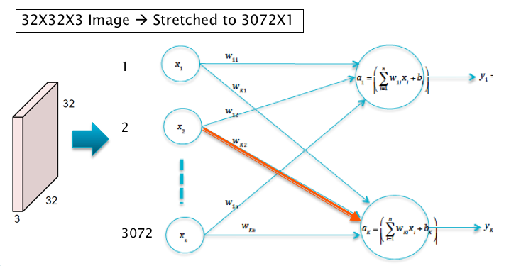
Figure 12.1: Image Processing using Linear Models

In order to motivate the design of ConvNets, consider the case when the input consists of \(32\times 32\times 3\) CIFAR-10 images, which have to be classified into one of ten categories. Also assume that these images are processed by a Linear Model of the type discussed in Chapter 4 (see Figure12.1). The pre-activations \(a_k, i\le k\le 10\) in this model are given by \[ a_k = \sum_{i=1}^{3072} w_{ki} x_i + b_k,\ \ 1\le k\le 10 \] Recall that for each category \(k\), the weights \(w_{ki}, 1\le i\le 3072\) could be interpreted as a template or filter for the category \(k\) object, so that the classification operation can be interpreted as template matching with the input image, as shown in Figure 12.2.

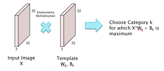
Figure 12.2: Classification as Template Matching

This template matching interpretation of Linear Filtering naturally leads to the following idea for improving the system: Instead of using a template that tries to match the entire image, why not use smaller templates that try to match objects in smaller local portions of the image. This has the following benefits: (a) Smaller templates need a smaller filter size and thus fewer parameters, and (b) Even if the object being detected moves around the image, the same template or filter can still be used, thus leading to translational invariance. This is the main idea behind ConvNets as illustrated in Figure 12.3.

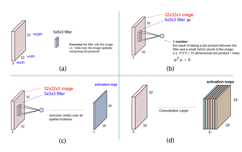
Figure 12.3: Illustrating Local Filters and Feature Maps in ConvNets

The main architectural aspects of ConvNets are illustrated in parts (a) - (d) of Figure 12.3:

Part (a) of Figure 12.3 illustrates the difference between template matching in ConvNets vs Feed Forward Networks as shown in Figure 12.2: ConvNets use a template (or filter) that is smaller than the size of the image in height and width, while the depths match. In the example shown in (a), a filter of size \(5\times 5\times 3\) is used for an image of size \(32\times 32\times 3\).
Part (b) shows the template matching operation in ConvNets. As shown here, the matching is done locally, for possibly overlapping patches of the image. At each position of the filter, the template matching is done using the following equation to compute the pre-activation \(a\) and activation \(z\):

\[\begin{equation} a = \sum_{i=1}^{75} w_{i} x_i + b, \end{equation}\] \[\begin{equation} z = f(a) \tag{12.1} \end{equation}\]

In this equation the pixel values \((x_1,...,x_{75})\), known as the Local Receptive Field, correspond to the local image patch of size \(5\times 5\times 3\) and changs as the filter is moved around (while the filter values \(w_i\) and \(b\) remain unchanged). Note that the filter now only has \(5\times 5\times 3 + 1 = 76\) parameters, as opposed to the \(32\times 32\times 3 + 1 = 3073\) parameters that were needed for the filter in Figure 12.2. Both the filter as well as the local image patch are 3-D structures, also called tensors, though the multiplication in Equation (12.1) uses a stretched out vectorized versions of the two tensors.

Part (c) of the figure shows the filter being moved across the image, and at each position Equation (12.1) is used to compute a new value of \(z\), and this generates a matrix of size \(28\times 28\). This matrix is known as an Activation Map (also called a Feature Map). This operation of sliding the filter across the image, while computing the dot product (12.1) at each position, is called a convolution. Using the same Filter for all the nodes in the Activation Map implies that all nodes in the Map are tuned to detect the same feature in the Input Layer, only at different positions in the image. This leads to the conclusion that ConvNets possess the property of Translational Invariance, i.e., they are able to detect objects irrespective of their location in the image.
Note that so far we have used a single filter which is only capable of detecting a single pattern in the input image. If we wish to detect multiple patterns, then we need multiple filters, each of which results in its own Activation Map, as shown in Part (d) of Figure 12.3. For example, Activation Map 1 may detect horizonal edges while Activation Map 2 detects vertical edges etc. As shown, a Hidden Layer in ConvNets consists of a stack of Activation Maps.

The filter in Fully Connected Deep Feed Forward Networks spans the entire input plane, which means that it is looking for patterns that span the entire image. However, real world images are built from smaller patterns that rarely span the entire image plane. Hence, by reducing the size of the filter, Convnets are better positioned to detect smaller shapes, which are then built hierarchically into bigger shapes and objects as we go deeper into the network. Also the Translational Invariance property ensures that the shape is detected irrespective of its location in the image plane.

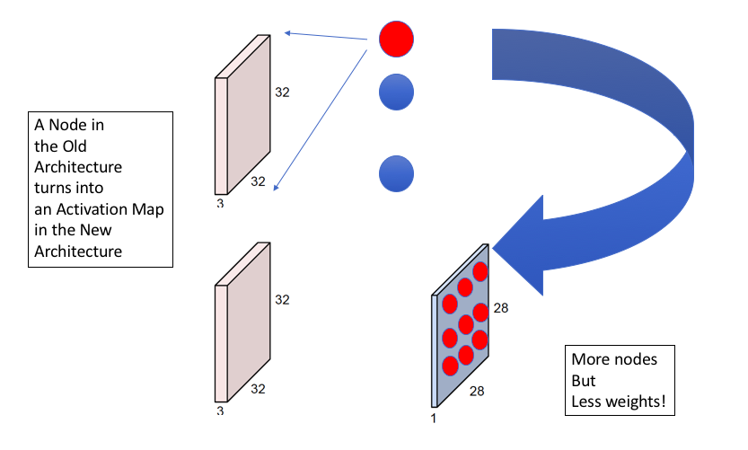
Figure 12.4: Relation between ConvNets and Deep Feed Forward Networks

Figure 12.4 illustrates another way to contrast ConvNets with Fully Connected Feed Forward networks. The top part of the figure shows a Fully Connected Feed Forward Network with the input image and the nodes in the first Hidden Layer. A node in this Hidden Layer is activated if it detects a particular pattern in the image, with each node looking for a different pattern. As shown in the bottom half of the figure, with ConvNets, each of the Hidden Layer nodes is replaced by an Activation Map with multiple “sub-nodes”. The activation value at each sub-node in an Activation Map is computed using a local filter which looks for the same pattern in different parts of the image. Hence in general we need as many Activation Maps in a ConvNet as there are nodes in a Hidden Layer of a Fully Connected Feed Forward Network. This figure also illustrates that ConvNets reduce the number of weights in the model at the expense of increasing the number of nodes. The increase in nodes causes the cost of computation to go up, but this is a worthwhile tradeoff to make since the reduction in the parameters makes the model easier to train with a smaller number of training examples.

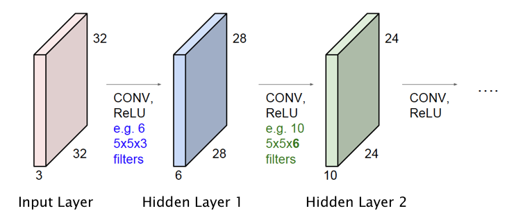
Figure 12.5: ConvNet with Multiple Hidden Layers

So far we have only described the operation of the Input Layer and the first Hidden Layer of the ConvNet. However it is straightforward to extend this design to multiple Hidden Layers, as shown in Figure 12.5. Just as in Fully Connected Deep Feed Forward Networks, Activation Maps in the initial hidden layers detect simple shapes, which are then built upon by the later layers to detect more complex shapes. The following hyper-parameters have to be chosen with each additional layer:

The number of Activation Maps to be used in the Hidden Layer
The size of the Filter and the Stride size (defined below), to be used to compute the Activations.

In the example in Figure 12.5, we added a second Hidden Layer with 10 Activation Maps, that are generated using a filter of size \(5\times 5\times 6\). Note that the depth of this filter is not a free variable since it has to equal to the number of Activation Maps in the previous layer.

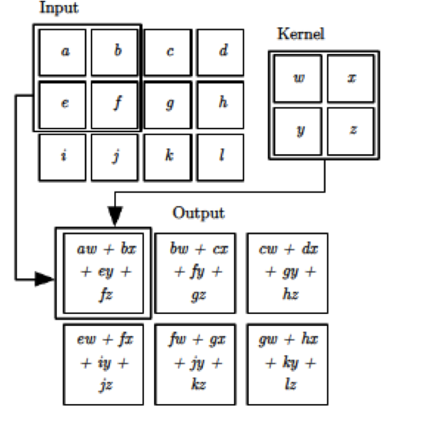
Figure 12.6: The Convolution Operation

The computations carried out to generate an Activation Map are shown in greater detail in Figure 12.6. It shows a Filter of size \(2\times 2\), operating on an input of size \(3 \times 4\) (without the depth dimension). In order to generate the activations, the filter is moved by one pixel at a time, horizontally and vertically, which results in an Activation Map of size \(2\times 3\). As we slide the \(2\times 2\) patch across the Input Layer, we compute a dot product of the activations in the Local Receptive Field with the filter weights. An important parameter used in this process is called the Stride, denoted by \(S\), and is defined as the number of pixels by which the filter is moved after each computation, either horizontally or vertically. Note that the example in Figure 12.6 corresponds to \(S = 1\).

Assuming that the \(r^{th}\) Hidden Layer is processed using a filter of size \(L\times W\times D\), note that this filter requires \(L \times W \times D + 1\) parameters. However, since the same filter is used for all the nodes in the Layer \(r+1\) Activation Map, it results in a huge reduction in the number of parameters needed to describe ConvNets. Since each Activation Map in Layer \(r+1\) requires its own filter, so that if there are \(C\) such Maps (i.e., Layer \(r+1\) is of depth \(C\)), then the total number of parameters needed is given by \(C \times (L \times W \times D + 1)\).

In order to appreciate the scale of the reduction in number of parameters due to shared filters, consider a ConvNet with Input Layer consisting of \(32\times 32\times 3\) images and containing a Hidden Layer with 20 Activation Maps generated using \(5 \times 5\) filters. Since each Activation Map requires \(5 \times 5\times 3+1=76\) filter parameters, \(76 \times 20 = 1520\) parameters are sufficient to generate the Hidden Layer. On the other hand, in a Fully Connected Deep Feed Forward architecture with \(32\times 32\times 3 = 3072\) nodes in the Input Layer and 20 nodes in the Hidden Layer, a total of \(3072\times 20+20 = 61,460\) parameters are needed.

Putting the concepts of Local Filtering and Parameter Sharing together, we now obtain an expression for the activations in a ConvNet using tensor notation. Define the following:

\(w_{lm}^{pq}(r)\): The value at position \(lm\) for the \(F \times F\) Filter that connects the \(p^{th}\) Activation Map of layer \(r\) with the \(q^{th}\) Activation Map of later \(r+1\). Note that these weight matrices together constitute a tensor object.
\(z_{jk}^{q}(r), a_{jk}^{q}(r)\): The activation and pre-activation at position \(jk\) of the \(q^{th}\) Activation Map in the \(r^{th}\) layer.
\(a_{jk}^{pq}(r)\): The portion of the pre-activation at position \({jk}\) of the \(q^{th}\) Activation Map in the \(r^{th}\) layer, which is due to the \(p^{th}\) Activation Map of the \((r-1)^{th}\) layer.
\(D_r\): Depth of the \(r^{th}\) layer.
\(b^{q}(r)\): The bias parameter associated with the \(q^{th}\) Activation Map in Layer \(r\).

The formula for the activations for the case \(S=1\), is then given by:

\[ \begin{equation} a_{jk}^{pq}(r+1) = \sum_{l=0}^{F-1}\sum_{m=0}^{F-1} w_{lm}^{pq}(r+1) z_{j+l,k+m}^p(r) \end{equation} \]

\[ \begin{equation} a_{jk}^{q}(r+1) = b^{q}(r+1)+\sum_{p=1}^{D_r}a_{jk}^{pq}(r+1),\ \ 1\le q\le D_{r+1} \end{equation} \]

\[\begin{equation} z_{jk}^{q}(r+1) = f(a_{jk}^{q}(r+1)) \tag{12.2} \end{equation}\]

where \(f\) is the Activation Function.

12.2 Pooling

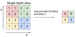
Figure 12.7: Pooling (http://cs231n.github.io/convolutional-networks/)

In addition to the Convolution operation described above, ConvNets also feature an operation called Pooling (see Figure 12.7). Pooling usually occurs after a Convolutional Layer, and can be described as condensing the information from that layer into a smaller number of activations. As shown in the figure, Pooling involves replacing a set of activations within a region of the Activation Map (which is just like a Local Receptive Field), by a single number. Usually the maximum of the activation values in the Local Receptive Field is used for pooling (called max-pooling), but other functions can also be used, such as the \(L_1\) or \(L_2\) norm. Unlike in Local Receptive Fields used in Convolutions, the corresponding fields used for the Pooling operation do not overlap. Note that the addition of Pooling does not introduce any new parameters to the ConvNet and the total number of parameters in the model are reduced considerably due to this operation.

In order to understand the Pooling operation, note that the numbers in an Activation Map that results from the Convolution operation, correspond to the likelihood of whether a particular shape or pattern is present in various locations in the previous layer. By doing Pooling right after Convolution, we throw away some of that information, which is the same as saying that the network does not care about the exact location of a pattern, it only needs to know whether the pattern is present or not. It should also be mentioned that as more processing power becomes available, some modern ConvNets, such as ResNet and the Google Inception Network, no longer incorporate Pooling in their design.

12.3 A Complete ConvNet

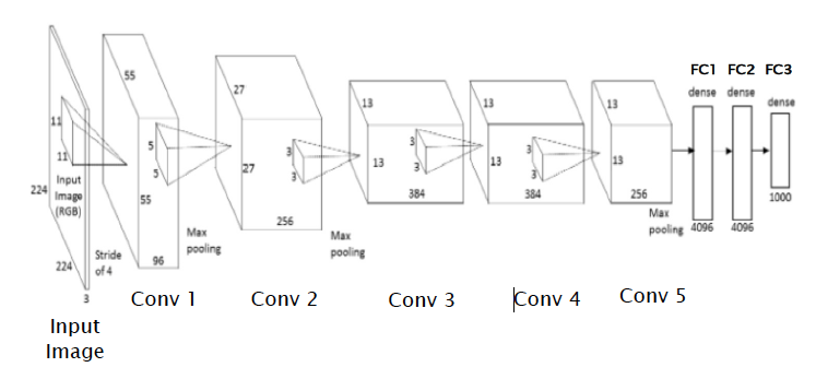
Figure 12.8: A Complete ConvNet

Figure 12.8 puts all the elements of a ConvNet together to come up with a network for the case when the input consists of \(224 \times 224\times 3\) pixel ILSVRC images. The figure shows a ConvNet called AlexNet which won the ILSVRC 2012 challenge. This network consist of the following:

Five convolutional layers
Three Max Pooling Layers, which occur after the first, second and fifth convolutional layers respectively.
Two Fully Connected Feed Forward Layers, consisting of 4096 nodes each, that are placed after the convolutional layers.
An Output Layer with 1000 nodes, corresponding to the 1000 categories that the input image can belong to.
The Filters vary from size \(11\times 11\) used for the first convolution, to size \(3\times 3\) used for the fifth convolution.

At a high level, the convolution operation changes the representation of an image, starting from raw pixels at one end, to higher level representations using successive layers of filtering. In abstract space, as the system goes through multiple Convolutional Layers, it is basically performing non-linear transformations so that images with similar objects are clustered closer to each other in the higher level transform space. This enables the classification operation to happen using a simple linear classifier in the final layer of the network. The Fully Connected layer that is just prior to the Output Layer, is called the FC2 layer, and it contains a 4096-dimensional representation of the input image. It is often used in other Deep Learning architectures that need a high level image representations (such as for image captioning, which is discussed in Chapter 13). Adding Fully Connected layers to a ConvNet leads to an enormous increase in the number of parameters, hence another trend in modern ConvNets is to replace them with layer that uses “Average Pooling”, as discussed later in this chapter.

12.4 Sizing ConvNets

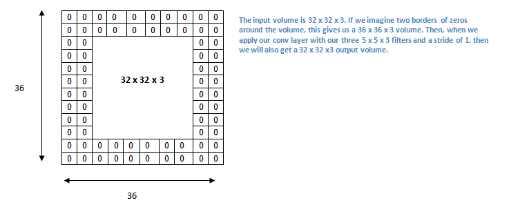
Figure 12.9: Zero Padding (http://bakeaselfdrivingcar.blogspot.com/2017/08/project-2-traffic-sign-recognition-with.html)

The size (or volume) of a Convolutional Layer in a ConvNet is related to the volume of the prior Convolutional Layer, as well as the size of the Filter used in the convolution operation, and in this section we give some simple expressions that can be used to connect the two. Before we launch into this topic, we introduce another important parameter used in ConvNet design, namely the Zero-Padding used during convolution, which we denote as \(P\). Zero-Padding does the following: Instead of processing an input of size \(L \times W\), we add one or more layers of zeroes around it, in both the dimensions. Hence if \(P=1\) then only a single Zero-Padding layer is added, while two layers are added for the case \(P=2\) (see Figure 12.9 for an illustration of the case \(P=2\)).

We will use the following notation:

\(L_r\), \(W_r\), \(D_r\): Length, Width and Depth dimensions of the volume in layer \(r\)
\(F_r\): Size of the Filter used when going from layer \(r\) to \(r+1\).
\(P_r\): Amount of Zero Padding used for layer \(r\).
\(S_r\): The Stride size used in the layer \(r\) to layer \(r+1\) filter.

It can then be shown that \[ W_{r+1} = \frac{W_r-F_r+2P_r}{S_r}+1 \] and \[ L_{r+1} = \frac{L_r-F_r+2P_r}{S_r}+1 \]

Also, with parameter sharing, \(F_r\times F_r\times D_r + 1\) weights are required per Activation Map in layer \(r+1\), for a total of \(D_{r+1}\times (F_r \times F_r \times D_r +1)\) weights and \(D_{r+1}\) biases in total.

For example consider the case when the input layer is of size \(7\times 7\), and a \(3\times 3\) filter with stride 1 is used with no zero padding. Then \(W_{r+1}=\frac{7-3+0}{1}+1 = 5\), so that the output Activation Map is of size \(5\times 5\). As another example of the application of this formula, consider the following example: \(W_r=10, F_r= 3, S_r=2\) with no zero padding, so that \(P_r=0\). Then applying the above formula it follows that \(W_{r+1} = 4.5\), which being a non-integer implies that it is not possible to fit an integer number of nodes in layer \(r+1\). We can change the stride to \(S_r=1\) which leads to \(W_{r+1}=5\), thus resulting in a valid architecture.

In modern ConvNet design, zero padding is used most often to ensure that the volume sizes remain unchanged as we move deeper into the network, in other words we would like that \(W_{r+1}=W_r, L_{r+1}=L_r, D_{r+1}=D_r\). From the above equation, this can be ensured if the stride \(S_r=1\) and the zero padding \(P_r\) is chosen to be:

\[ P_r = \frac{F_r - 1}{2} \]

The most ConvNet filter sizes are \(F_r = 3\) and \(F_r = 5\), which results in \(P_r = 1\) and \(P_r = 2\) respectively. As we will see later in this chapter, some of the advanced ConvNet designs such as the VGGNet and the ResNet keep the size of the volumes fixed in their Convolutional Layers, which helps in producing networks with hundreds of layers. In the absence of this feature, the volume sizes progressively decrease as we move deeper in the network, thus limiting the number of Hidden Layers to much smaller values.

As we will see later, early ConvNet designs featured bigger Filters, such as \(11\times 11\) or \(7\times 7\), in their first few layers. However in more recent designs, it has been discovered that using smaller \(3\times 3\) filters, even in the first layer, leads to better performance, as well as a reduction in the number of parameters. This aspect of ConvNet design is explored more fully in Section 12.6.

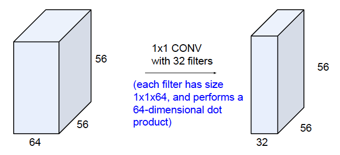
Figure 12.10: Illustrating 1X1 Filters

Some additional considerations in sizing ConvNets are:

The depth \(D_r\) is usually chosen to be a power of \(2\) for computational reasons: Numerical routines used in the calculations work more efficiently in this case.
Several modern ConvNets use Filters of size \(1\times 1\). At first glance these may not make sense, but note that because of the depth dimension, a \(1\times 1\) Filter still involves a dot product with weights associated with the depth dimension and the corresponding activations across them. As shown in Figure 12.10, this can be used to compress the number of layers in a ConvNet. This is a very useful operation and is frequently used in modern ConvNets to reduce the number of parameters or the number of operations required.

12.4.1 Sizing the Pooling Layer

If Layer \(r+1\) is a Pooling Layer, then the following formulae hold (using the same notation as in the prior section):

\[ W_{r+1} = \frac{W_r-F_r}{S_r} + 1 \]

\[ H_{r+1} = \frac{H_r-F_r}{S_r} + 1 \]

\[ D_{r+1} = D_r \]

Note the following:

The Pooling Layer does not lead to the introduction of new parameters.
It is not common to use Zero Padding as part of Pooling, hence the absence of the \(P_r\) term in the above equations.
Common numbers used for Pooling are \(F_r = 2, S_r = 2\) or \(F_r = 3, S_r = 2\).

12.5 Training ConvNets

ConvNets can be trained using a modified version of the Backprop algorithm that was described in Chapter 6. The modification, which is necessary due to the fact that multiple nodes now share the same weight parameters, is as follows:

The forward pass of the Backprop algorithm is as before, during which we compute all the node activations \(z_{jk}^{q}(r)\) using the formula (12.2).
During the backward pass we compute the gradients \(\delta_{jk}^{q}(r)\) for each node as before.
The final computation of the gradient of the Loss Function with respect to the weight parameters is modified as follows: The gradient with respect to a weight parameter is computed as the sum of the gradients of all the connections that share the same weight.

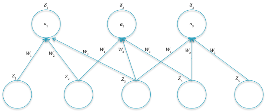
Figure 12.11: Computing Gradients in ConvNets

In order to justify the last rule, consider Figure 12.11: Focusing on the weight \(w_1\), note that the gradient \(\frac{\partial L}{\partial w_1}\) depends on \(w_1\) through the pre-activations \(a_1, a_2, a_3\) due to the parameter sharing property (this is in contrast to Fully Connected Networks where the dependence was only on \(a_1\)). As a result, using the chain rule we obtain:

\[ \frac{\partial L}{\partial w_1} = \frac{\partial L}{\partial a_1}\frac{\partial a_1}{\partial w_1} + \frac{\partial L}{\partial a_2}\frac{\partial a_2}{\partial w_1} + \frac{\partial L}{\partial a_3}\frac{\partial a_3}{\partial w_1} \] Noting that \(\frac{\partial a_i}{\partial w_1}=z_i,i=1,2,3\) and \(\frac{\partial L}{\partial a_i}=\delta_i\), we obtain \[ \frac{\partial L}{\partial w_1} = z_1\delta_1 + z_2\delta_2 + z_3\delta_3 \] The process of generating the gradients \(\delta^{(r)}\) at layer \(r\), from the gradients \(\delta^{(r+1)}\) at layer \(r+1\) was fairly straightforward in Fully Connected networks, and corresponded to a multiplication by the transpose \(W^T\) of the weight matrix. In the case of ConvNets, the corresponding operation is a little more involved, and proceeds by multiplication by the transpose of the filter matrix. In order to do this efficiently using matrix multiplication, we have to pad the Activation Map (made up of gradients) by zeroes. The reader can verify this by running the operations in Figure 12.11 backwards.

12.6 Small Filters in ConvNets

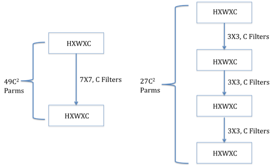
Figure 12.12: Single 7x7 Filter vs Three 3x3 Filters

As ConvNet architectures have matured, one of the features that has changed over time is the filter design. Early ConvNets such as AlexNet used large \(7 \times 7\) Filters in the first convolutional layer. However, a stack of \(3 \times 3\) Filters is a superior design to the single \(7 \times 7\) Filter for the following reasons (see Figure 12.12):

The stacked \(3 \times 3\) design uses a smaller number of parameters: Using the formula for number of parameters in a ConvNet developed in Section 12.4, it follows that the \(7 \times 7\) Filter uses \(C \times (7 \times 7 \times C + 1)=49 C^2 + C\) parameters (since each Filter uses \(7 \times 7 \times C + 1\) parameters, and there are C such Filters). In comparison the stacked \(3 \times 3\) design uses a total of \(3 \times C \times (3 \times 3 \times C + 1)=27 C^2 + 3C\) parameters, i.e., a 45% decrease.
The stacked \(3 \times 3\) design incorporates more non-linearity, it has 4 ReLU Layers vs the 2 ReLU Layers in the \(7 \times 7\) case, which increases the system’s modeling capacity.
The stacked \(3 \times 3\) design results in less computation.

The better performance with smaller filters can be explained as follows: The job of a filter is to capture patterns within the Local Receptive Field and patterns at a finer level of granularity can be captured with smaller filters. Also as we stack up the layers, filters at the deeper levels progressively capture patterns within larger areas of the image. For example consider the case of the stacked \(3 \times 3\) Filters in Figure 12.12: While the first \(3 \times 3\) Filter scans patches of size \(3 \times 3\) in the input image, it can be easily seen that the second \(3 \times 3\) filter effectively scans patches of size \(5 \times 5\), and the third \(3 \times 3\) Filter scans patches of size \(7 \times 7\) in the input image. Hence even though the filter size is unchanged as we move deeper into the network, they are able to capture patterns in progressively larger sections of the input image.

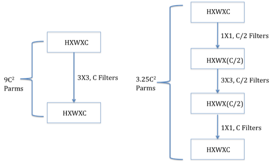
Figure 12.13: Illustration of 1x1 Filters

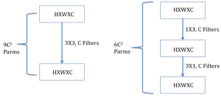
Figure 12.14: Illusration of 1 imes 3 and 3 imes 1 Filters

It is in fact possible to reduce the number of parameters further by using \(1 \times 1\) and \(1 \times n\) filters, as shown in Figures 12.13 and 12.14.

The architecture in Figure 12.13 illustrates the use of \(1 \times 1\) filters in ConvNets. As shown there, the first \(1 \times 1\) filter is used in conjuction with a reduction in depth to \(C/2\). The \(3 \times 3\) filter then acts on this reduced depth layer, which gives us the reduction in parameters, and this is followed by another \(1 \times 1\) filter than expands the depth back to \(C\). It can the shown that this filter architecture reduces the number of parameters from \(9 C^2\) to \(3.25 C^2\) (ignoring the bias parameters).
Figure 12.14 shows how \(1 \times 3\) and \(3 \times 1\) filters can be used in series with a \(3 \times 3\) filter to reduce the number of parameters from \(9C^2\) to \(6C^2\).

12.7 ConvNet Architectures

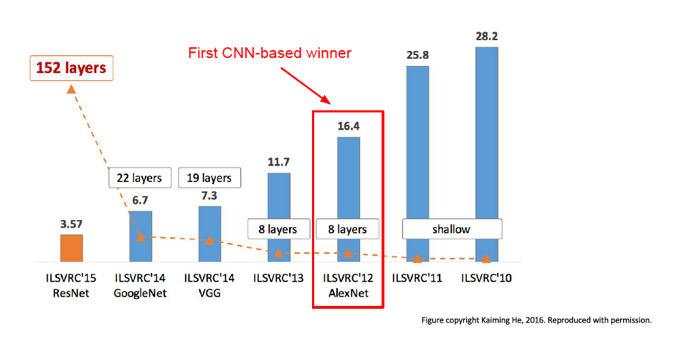
Figure 12.15: Evolution of Network Size and Error Rate in ILSVRC

We briefly survey ConvNet architectures starting with the first ConvNet, LeNet5, whose details were published in 1998. Starting with AlexNet in 2012, ConvNets have won the ImageNet Large Scale Visual Recognition Challenge (ILSVRC) image classification competition run by the Artificial Vision group at Stanford University. ILSVRC is based on a subset of the ImageNet database that has more than 1+ million hand labeled images, classified into 1,000 object categories with roughly 1,000 images in each category. In all there are 1.2 million training images, 50K validation images and 150K testing images. If an image has multiple objects, then the system is allowed to output upto 5 of the most probably object categories, and as long as the the “ground-truth” is one of the 5 regardless of rank, the classification is deemed successful (this is referred to as the top-5 error rate).

Figure 12.15 plots the top-5 error rate and (post-2010) and the number of hidden layers in DLN architectures for the past seven years. Prior to 2012, the winning designs were based on traditional ML techniques using SVMs and Feature Extractors. In 2012 AlexNet won the compeitition, while bringing down the error rate signficantly, and inaugurated the modern era of Deep Learning systems. Since then, the error rates have come down rapidly with each passing year, and currently stand at 3.57%, which is better than human-level classification. At the same time, the number of Hidden Layers has increased from the 8 layers used in AlexNet, to 152 layers in ResNet which was the winner in 2015. This is when the machines outpaced humans in accuracy.

In this section our objective is to briefly describe the architecture of the winners from the last few years, namely: AlexNet (2012), ZFNet (2013), VGGNet (2014), Google InceptionNet (2014) and ResNet (2015). The first three are “classical” ConvNet designs of the type we have seen in this chapter, with multiple Convolutional, Pooling, and Fully Connected layers arranged in a linear stack. The Google Inception Network and ResNet have diverged from some of the basic tenets of the first ConvNets, in particular:

Linear Stacking of Layers: The first ConvNets stacked layers linearly on top of each other, however the Google Inception Network does not follow this design. Instead it uses a tree like structure in which the system simultaneously uses multiple filters of different sizes.
Superposition of Signals from Multiple Layers: Unlike the first Convnets in which the input to Layer \(r+1\) is entirely from Layer \(r\), the ResNet architecture superposes the signals from multiple layers.
Use of the Pooling and Fully Connected Layers: Neither Google Inception nor ResNet use the Pooling or Fully Connected Layers.

These architectures are described in greater detail next.

12.7.1 LeNet5 (1998)

LeNet5 was the first ConvNet, it was designed by Yann LeCun and his team at Bell Labs, see LeCun et al. (1998). It had all the elements that one finds in a modern ConvNet, including Convolutional and Pooling Layers, along with the Backprop algorithm for training (Figure 12.16). It only had two Convolutional layers, which was a reflection of the smaller training datsets and processing capabilities available at that time. LeCun et.al. used the system for handwritten signature detection in checks, and it was successfully deployed commercially for this purpose.

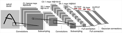
The LeNet5 Architecture (see Figure 2 in @Lecun98gradient-basedlearning)

Figure 12.16: The LeNet5 Architecture (see Figure 2 in LeCun et al. (1998))

As shown in Figure 12.16, the system uses two Convolution layers with \(5 \times 5\) Filters and Stride \(S=1\), and two Pooling layers with \(2 \times 2\) Filters and \(S=2\). The system reduces the input \(32 \times 32\) images with 3 RGB layers into 16 Activation Maps of size \(5 \times 5\) at the end of the second pooling operation, before outputting the result into the Fully Connected part of the design.

12.7.2 AlexNet (2012)

After the pioneering work done in LeNet5, progress in ConvNets lay dormant for more than a decade. It was held back by the following issue: In order to train larger ConvNets with millions of parameters, it was necessary to have a large training dataset with correspondingly millions of images (this is required in order to prevent overfitting, see Chapter 8 for an explanation). Image datasets of this size did not exist until about 2010, when the ImageNet dataset was released.

AlexNet is responsible for the explosion in interest in DLNs in the last few years.This network won the ILSVRC competition in 2012 by a wide margin compared to its nearest rival which was based on SVMs (it had a 15.4% top-5 error rate vs 26.2% for the next lowest network), and this opened up the eyes of the ML community to the potential of DLNs. The architecture of AlexNet (Krizhevsky, Sutskever, and Hinton 2012) was very similar to that of LeNet5, with the following exceptions (Figure 12.8):

AlexNet replaced the tanh() activation function used in LeNet5, with the ReLU function and also the MSE loss function with the Cross Entropy loss.
AlexNet used a much bigger training set. Whereas LeNet5 was trained on the MNIST dataset with 50,000 images and 10 categories, AlexNet used a subset of the ImageNet dataset with a training set containing 1+ million images, from 1000 categories.
AlexNet used Dropout regularization (= 0.5) to combat overfitting (but only in the Fully Connected Layers). It also used a Normalization Layer, that is no longer used in ConvNets since it does not improve the performance significantly.

AlexNet was able to use a training set which was larger by two orders of magnitude, without a corresponding increase in training time, by exploiting the power of GPUs. It used two GTX 580 GPUs for 5-6 days to complete the training phase.

AlexNet used 5 Convolutional layers (vs 2 used in LeNet5), and it used a similar combination of Convolutional and Pooling Layers followed by 3 Fully Connected Layers. The input into the system consisted of \(227 \times 227 \times 3\) images, which are then processed by the first convolutional layer with 96 Activation Maps using \(11 \times 11\) filters with \(S=4, P=0\). The system has \(4\) more Convolutional layers, consisting of a \(5 \times 5\) Filter followed by three \(3 \times 3\) Filters. The number of Activation Maps in the last Convolutional layer is increased to 256 before the activations are fed into the Fully Connected Layers.

AlexNet had a total of 60 million parameters, which was still much more than the number of training images available. In order to prevent overfitting, the system used Data Augmentation techniques to produce additional test images, thus boosting the Test dataset to 15 million images.

12.7.3 ZFNet (2013)

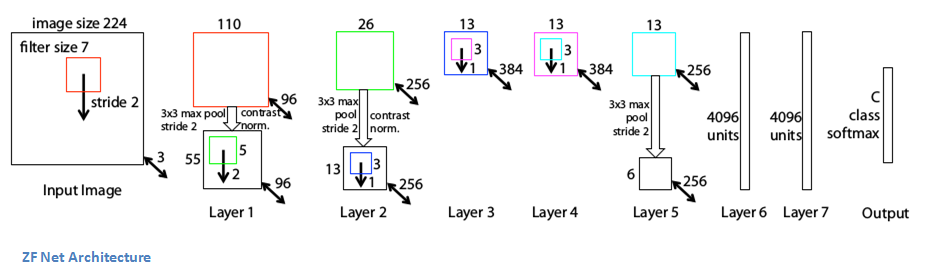
The ZFNet Architecture (Figure 3 in @DBLP:journals/corr/ZeilerF13)

Figure 12.17: The ZFNet Architecture (Figure 3 in Zeiler and Fergus (2013))

ZFNet, which was designed by Zeiler and Fergus (2013), won the ILSVRC competition in 2013 by achieving a 11.2% top-5 error rate. The architecture was a slight modification to AlexNet, with the following differences (Figure 12.17):

Instead of using \(11 \times 11\) Filters in the first Convolutional layer, ZFNet used a \(7 \times 7\) Filter with \(S=2\). A smaller filter size helps to pick image features at a finer level of resolution.
ZFNet increased the number of Activation Maps in the 3rd, 4th and 5th Convolutional layers from \((385,384,256)\) to \((512, 1024, 512)\), which increased the number of features that the network is capable of detecting.

12.7.4 VGGNet (2014)

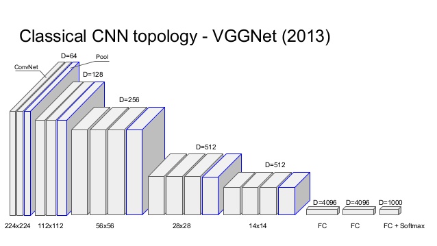
Figure 12.18: The VGGNet Architecture

Simonyan and Zisserman (2014) created a network which reduced the top-5 ILSVRC error rate to 7.3% (Figure 12.18). The main innovations in the network, called VGGNet, are the following:

VGGNet increased the number of layers to 19 layers (16 Convolutional + 3 Fully Connected), as opposed to the previous designs that were limited to 8 such layers.
VGGNet considerably simplified the ConvNet design, by repeating the same smaller convolution filter configuration 16 times: All the filters in VGGNet were limited to \(3 \times 3\), with stride and padding of 1, along with \(2 \times 2\) maxpooling filters with stride of 2. Since these smaller filters are used in a series of 2 or 3 consecutive convolutional layers, the net effect is that of using a single \(5 \times 5\) or \(7 \times 7\) filter, but with the advantage of a smaller number of parameters and increased model non-linearity, as explained in Section 12.6.

An interesting fact about about VGGNet is that it has a total of 144 million parameters, of which about 124 million parameters are used in the final 3 Fully Connected layers. Hence it would be nice if the Fully Connected layers could be eliminated (without affecting performance), and this step was carried out in subsequent architectures which replaced the first Fully Connected layer with a layer of 512 nodes using a technique called Average Pooling. In order to understand how Average Pooling works, consider the last Convolutional Layer in VGGNet which has dimension \(7 \times 7 \times 512\). If we connect this to a fully connected layer with 4096 nodes, then we would need a total of \(7 \times 7 \times 512 \times 4096=102,760,448\) parameters. Average Pooling on the other hand averages out the plane of \(7 \times 7=49\) activations in each of the 512 Activations Maps, and thus converts the entire block of \(7 \times 7 \times 512\) nodes to a linear layer of 512 nodes. This technique was used in the next two architectures that we describe, the Google Inception Network and the ResNet.

Even though VGGNet did not win the ILSVRC competition in 2013, it came close to doing so, and its simple and elegant design has been influential in subsequent ConvNet architectures. The main lesson from VGGNet was the classical ConvNet design of the LeNet5/AlexNet type can be substantially improved by increasing the number of Convolutional Layers and by using smaller filters.

12.7.5 Google Inception Network (2014)

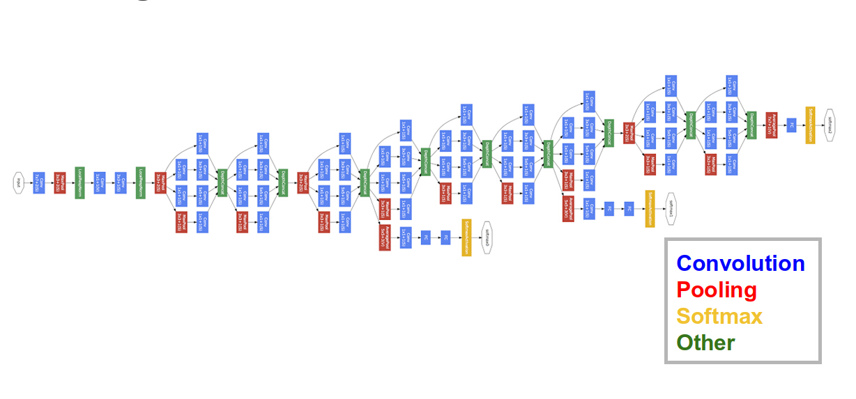
Figure 12.19: The Google Inception Architecture

Along with VGGNet, the Google Inception Network (Figure 12.19) competed in the 2014 ILSVRC competition, see Szegedy, Ioffe, and Vanhoucke (2016). It did slightly better than VGGNet (6.7% top 5 error rate as compared to 7.3% for VGGNet), but at the cost of a more complex architecture. The Inception Network was the first design that moved away from the linear stacking of convolutional and pooling layers. It was able to considerably reduce the number of parameters by using the following design innovations:

Elimination of all the fully connected layers and the use of Average Pooling, as a result of which the system uses only 5 million parameters.
Introduction of the Inception Module (see Figure 12.20): The base Inception module is repeated multiple times to create the network.

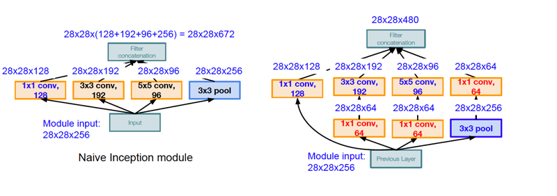
Figure 12.20: The Inception Module

The reasoning behind the design of the Inception Module is as follows: As the LHS of Figure 12.20 shows, the basic idea of the Inception module is to process the input data using multiple filters in parallel, before concatenating all their Activation Maps together and forming the input to the next stage. The Inception module uses four different types of convolutional engines: \(1 \times 1\), \(3 \times 3\), \(5 \times 5\), and \(3 \times 3\) with max-pooling. The smaller convolutions extract features at a finer level of detail, while the larger convolutions deal with features at a coarser level. However there is a problem associated with the architecture on the LHS: After the Activation Maps on all the four branches are concatenated, it results in 672 Activation Maps at the output of the module! As we add more modules, this will clearly result in an explosion in the number of Activation Maps, thus making the architecture infeasible. Another problem with the architecture is the exteremely large number of numerical operations required to compute the activations.

The solution to these problems is shown on the RHS of Figure 12.20: We add three Activation Maps to the design, that are generated using \(1\times 1\) convolutions. The \(1\times 1\) convolution in series with the Pooling layer reduces the number of Activation Maps in that branch from 264 to 64, which reduces the total number of Activation Maps at the output to 480. In addition two more \(1\times 1\) convolutions are added to the \(3\times 3\) and \(5\times 5\) filter branches to compress the number of input Activation Maps to 64, before they are processed by the larger filters. This helps to reduce the number of numerical computations required from 854 million to 358 million.

The Inception design aligns with the intuition that visual information should be processed at different scales and then aggregated so that the next stage can abstract features from different scales at the same time. The designers of the system also included a couple of extra output modules in the middle of the network (see Figure 12.19), in order to amplify the error signal propagating towards the initial portion of the network, since they were concerned that the large number of layers in the network will cause the error signal to fade by the time it gets to that part of the network.

12.7.6 ResNet (2015)

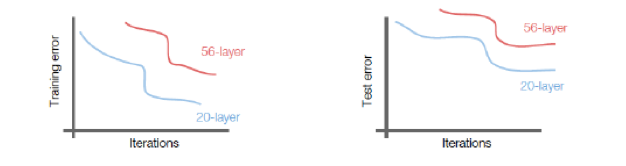
Figure 12.21: Variation of Training and Test Error with Number of Layers

ResNets (short for Residual Neural Networks) were introduced by He et al. (2015 a), and this design won the ILSVRC 2015 competition by a wide margin, achieving an error rate of 3.57%. ResNets have innaugurated the era of ultra-deep ConvNets, indeed the winning ResNet network came with 152 layers, an order of magnitude jump from the 22 layers in the previous year’s winner. The main architectural innovation in ResNets made such deep networks possible, and is based on the following insight: The number of layers in a ConvNet is constrained due to the fact that the error information propagating back during the backward phase of the Backprop algorithm, tends to get more and more diffused by the time it gets to the initial layers, due to multiplications with the weights and activations in the intervening layers. As a result the weights in the initial few layers are not modified in an optimal fashion during Gradient Descent. This effect is shown in Figure 12.21, which shows that both the Training and Test Error for a 56-layer network is higher when compared to that of a 20-layer network (which implies that the increase cannot be attributed to overfiting).

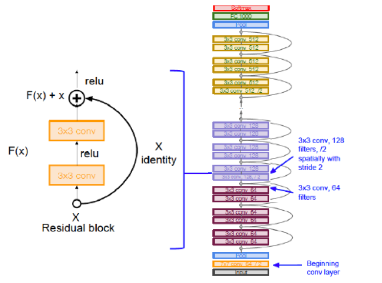
Figure 12.22: The ResNet Architecture

In order to overcome this problem, He et al. (2015 a) introduced a bypass link, as shown in LHS of Figure 12.22.

In the forward pass of Backprop, the bypass link enables the input signal to skip a few stacked Convolutional Layers, and then it is added to the output of these layers as shown. Note that the very first Convolutional Layer in the system is not bypassed. Hence one way to interpret this design is the following: The bypass enables the activation after the first convolutional layer to propagate all the the front of the network, while being modified by some delta (or residue) from each of the intervening bypassed layers. This design is based on the hypothesis that it is easier to optimize the residual mapping than to optimize the original, unreferenced mapping.
In the backward pass of Backprop, the bypass enables the error gradient information from the Output Layer of the network, to propagate without modifications by intervening layers, all the way to the first Convolutional Layer. Hence all the layers in the network are able to access the unfiltered error gradient information from the Output Layer, irerspective of the total number of layers in the network. This property enables ResNets to go Ultra-Deep without sacrificing performance.

Other interesting aspects of ResNets include the following:

The system makes extensive use of Batch Normalization, see Section 7.7, which is implemented at the end of every layer.
It uses a relatively large Learning Rate of 0.1 (Section 7.2), which is divided by 10 whenever the validation error paltaeaus during training. Such a large rate is made possible due to the use of Batch Normalization.
The system does not make use of Dropout normalization (Section 8.4.4). It is theorized that Dropout is not needed in the presence of Batch Normalization.
The system does not make use of Fully Connected layers at the end of the network.

ResNets are currently the state of the art in ConvNets and are used by default in practical cases.

12.8 Transfer Learning

When ConvNets are trained on image data, such as ImageNet, we have the luxury of having a database of millions of labeled images, which enables us to train fairly large networks with hundreds of layers to a high degree of accuracy. These networks, examples of which include ResNet, VGGNet, or Google InceptionNet, take multiple weeks to train, and involve huge amounts of advanced computing resources such as GPUs, to do so.

Practitioners often run into problems when there are not enough training examples to train such large networks, or if they don’t have access to the necessary computing resources for the particular problem that they are trying to solve. Fortunately there is a technique called Transfer Learning that enables us to develop accurate ConvNet models even without a lot of training data. Transfer Learning enables us to transfer the parameters learnt from training a model for Problem 1, to be re-used in the model for another Problem 2, provided the training dataset for Problem 2 is similar to that used for Problem 1.

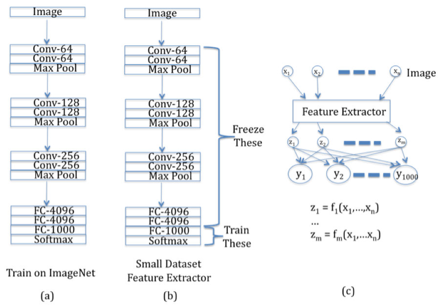
Figure 12.23: Illustration of Transfer Learning, Part 1

In order to understand how Transfer Learning works, consider Figure 12.23. Part (a) of the figure shows a traditional ConvNet, say ConvNet 1, which has been trained on a large dataset such as ImageNet. It has a mixture of Convolutional and Maxpool layers, which is followed by Fully Connected layers at the end of the network. In order to reuse the parameters learnt from this network, to another network, say Convnet 2, with a similar dataset which is much smaller in size, we do the following:

As shown in Part (b) of Figure 12.23, we freeze the parameters of ALL the layers of ConvNet 1, except for the Output Layer that is used for classification, and then use these parameters as a Feature Extractor in ConvNet 2. The reader may recall from Chapter 4 that ConvNet 2 corresponds to a simple Logistic Regression model with a Feature Extractor used in the Input Layer.
In order to complete ConvNet 2, we only need to find the weights of the connections between the Feature Extractor outputs \({z_i}\) and the Output Layer \({y_i}\), as shown in Part (c) of Figure 12.23. Since the number of weights are now much smaller, they can be estimated using the smaller dataset available for ConvNet 2.

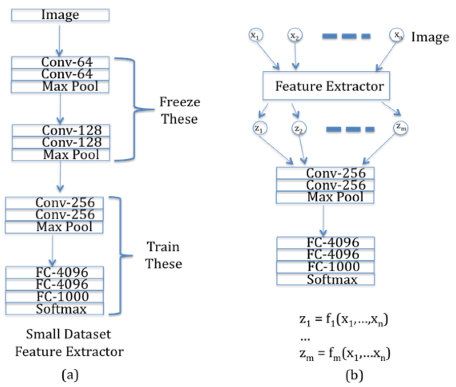
Figure 12.24: Illustration of Transfer Learning, Part 2

If larger datasets are available for Problem 2 (but which are still smaller than ImageNet in size), then the technique that was explained above, can be extended to networks with additional layers, as shown in Figure 12.24. In this case we reduce the number of frozen layers from ConvNet 1, so that ConvNet 2 now has additional layers that need to be trained. Once again the frozen layers in ConvNet 1 act as a Feature Extractor whose outputs are fed into the rest of the convolutional network.

Why does Transfer Learning work so well? A ConvNet trained on a large dataset such as ImageNet, learns to recognize generic patterns and shapes that also occur in non-ImageNet data. In addition, even non-image data, such as audiowave signals, can be classified well with the patterns that are learnt with ImageNet. A general rule of thumb is that the earlier Hidden Layers in the ConvNet contain the more generic portion that can be re-used in other contexts, and the model becomes more and more specific to the particular dataset, as we go deeper into the network.

In practice, researchers can save a large amount of time (and money), by not starting from scratch, but instead use an appropriate pre-trained model, when they start working on a new model. A large number of pre-trained ConvNet models, including all the models discussed in this chapter, are available as part of the “Model Zoo” in the CaffeNet ConvNet Library (https://github.com/BVLC/caffe/wiki/Model-Zoo).

12.9 Visualizing ConvNets

ConvNets seem to work very well and constitute a significant advance in neural network architecture. However their decision making process proceeds through complex non-linear computations that are opaque to humans. In order to gain more confidence in the output of these networks, it would be nice if we can get some insights into how they go about doing their job. The field of ConvNet Visualization attemtps to do this in various ways that are described in this section. In particular we will describe the following techniques:

Visualizing Local Filters: Using the template matching interpretation of image recognition, the shape of local filters can tell us the kind of objects the network is looking for.
Visualizing the last layer in the Feature Space: The Last Layer before the classification step represents the results of all the transformations on the original image, and hence visualizing its co-ordinates gives insights into the ConvNets’s operation.
Identifying Maximally Activating Patches in Images: This technique solves the following problem: Given a neuron that gets activated by an image, identify the portion of the image that it is reacting to.
Generating Images that Maximize Neuron Activations: This is the process of running the ConvNet backwards to generate images that maximize the activation at a chosen neuron.
Generating Images from Feature Vectors: This also involves running the ConvNet backwards, to generate images whose Feature Vectors match those from a sample image.

12.9.1 Visualizing Local Filters

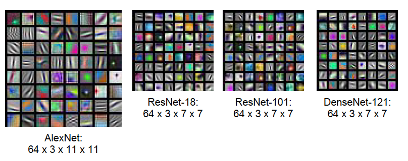
Figure 12.25: Visualization of the Filters in the first Hidden Layer

Consider a ConvNet, such as AlexNet, with 64 Activation Maps in the first Hidden Layer which are generated using 64 local filters of size \(3\times 11\times 11\). Each of these filters can be visualized by using the filter values to generate a \(11\times 11\) color image, and this is shown in Figure 12.25 for AlexNet as well as for a few other types of ConvNets. Using the template matching interpretation of local filtering, it follows that first Hidden Layer filters in all these networks are mostly looking for straight edges in various orientations. Hubel and Wiesel had discovered that the visual system in animals has a similar property, in that the first layer of neurons in the visual cortex is sensitive to the presence of edges in the image falling on the retina.

Unfortunately it is not possible to as readily visualize filters in the deeper layers of the network, due to the fact that they possess a depth of more than 3 and hence cannot be converted into a color image. Hence in order to understand what is happening in the deeper layers of the network, we rely on techniques described in the following sub-sections.

12.9.2 Visualizing the Proximity Property of Feature Space Representations

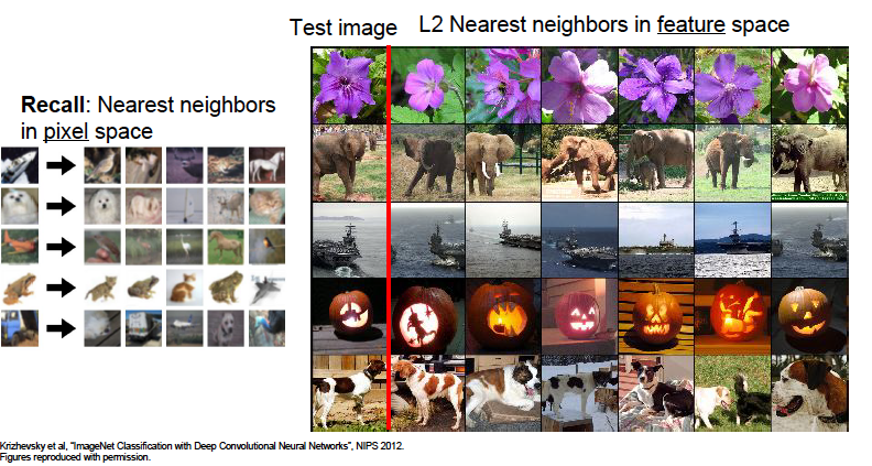
Figure 12.26: Visualization of the Images that are close in Feature Space

We have emphasized the fact that DLNs transform the representation of images from RGB pixels to a feature space representation that also carries semantic information, such that images that are in the same category tend to have representations that cluster together in feature space. This property can be verified by examining the L2 nearest neighbors for an image, as shown in the RHS of Figure 12.26. This figure shows the sample image in the first column on the left side of the figure, while the images in each row correspond to those whose feature space L2 distance is closest to the sample image in that row. The feature space representation is obtained as the activations of the FC2 Fully Connected layer in AlexNet (see Figure 12.8). We note the following:

Images whose pixel values are very different are nevertheless close to each other in feature space, thus verifying the semantic clustering property of DLNs.
On the other hand, relying on L2 nearest neighbors in pixel space is not a reliable way of clustering images, since it can result in images that are in different categories, as shown on the LHS of Figure 12.26.

12.9.3 Identifying Maximally Activating Patches in Images

Several times in this book, we have used the intuitive notion that the neurons in succesive layers in a DLN detect image features in an hierarchical fashion, with lower layers detecting simple features that are then used by the higher layers to detect more complex shapes. This intuition can be verified for ConvNets by using the concept of Maximally Activating Patches, which are defined as follows: Pick any node in a ConvNet, it can be one of the classification layer nodes whose activation is equal to the class-score of the corresponding category, or it can even be a neuron in one of the Activation Maps within a convolutional layer. Assuming that the input image is such that it results in a high activation value at the chosen node, i.e., the neuron reponds positively to some pattern that it detects in the image. Then the Maximally Activating Patch is defined to be the portion of the image that the neuron is responding to.

Maximally Activating Patches are identified by running the ConvNet backwards, which is actually a very important notion. Though originally proposed as a way to identify Maximally Activating Patches, the backwards operation has since been extended to tasks that involve generating new images from a trained ConvNet.

There are two main techniques that are used to run a ConvNet backwards:

DeConvNet
Guided Backpropagation

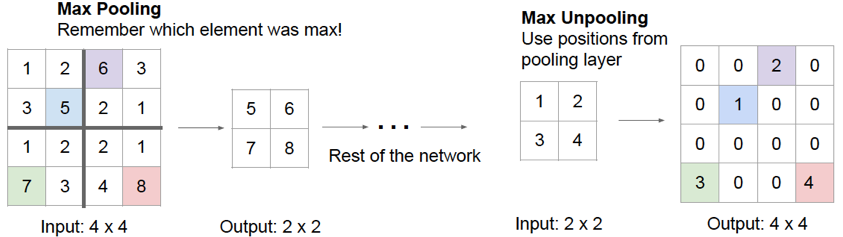
Figure 12.27: Backwards Propagation through Pooling Layers

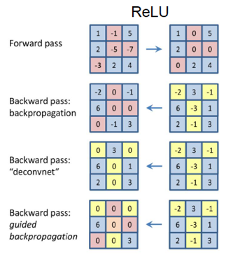
Figure 12.28: Backward through ReLU Non-Linearities

Both these techniques use the same computations for going backwards through Convolutional and Pooling layers, but differ in the way they pass through ReLU non-linearities. These operations are described next:

Backwards through Convolutional Layers: This operation is the same as that carried out by backpropagating gradients in the Backprop algorithm, and involves multiplication by the transpose of the Convolutional Filter. For example, consider the 1-D convolution shown in Figure 12.11. The backwards convolutions are given by: \[ z'_1 = w_1 a'_1,\\ z'_2 = w_2 a'_1 + w_3 a'_2,\\ z_3' = w_3 a'_1 + w_2 a'_2 + w_1 a'_3, \\ z'_4 = w_3 a'_2 + w_2 a'_3,\\ z'_5 = w_3 a'_3 \] where \(z'_i\) and \(a'_i\) are the backwards propagating activations and pre-activations respectively. These calculations can be extended to two dimensions and also be put in a matrix form by padding the higher layer Activation Map with zeros around the edges.
Backwards through Pooling Layers: This operation is referred to as “switching” and proceeds as follows: Carry out a forward pass through the network, and keep record of the positions at which the maximum activation in max-pooling occurs (see FIgure 12.27). In the backward pass, the incoming activation is placed in the “maximum activation” spot, while all the activations are set to zero. The reader may recall that this rule was derived in Chapter 6 in the section on Gradient Flow Calculus.
Backwards through ReLU Non-Linearities: As shown in Figure 12.28, there are multiple ways in which a ConvNet can be run backwards through ReLU non-linearities:
- The top row of the figure shows a Forward Pass through a ReLU non-linearity. It shows the negative pre-activations on the LHS being reset to zero in order to generate activation numbers on the RHS of the figure.
- The second row in the figure shows a backward pass through a ReLU for gradients using traditional Backprop: Recall that the ReLU non-linearity acts as a switch for the gradients during Backprop, so that the negative pre-activations (in the LHS of the top row) cause the gradients in the corresponding positions to go to zero.
- The third row in the figure shows the ReLU backward pass used in DeConvNets. When going backwards through a ReLU non-linearity, all negative values are set to zero, as shown. In contrast to Backprop and Guided Backprop (see below), the numbers flowing back during the DeConvNet operation should not be thought of as gradients, they should be regarded as “activations”" that are propagating backwards.
- The fourth row in the figure shows a backward pass for gradients used in Guided Backpropagation. When passing backwards through ReLU non-linearity, the negative gradients are set to zero, in addition to the gradients for whom the corresponding input activation is negative. Hence the Guided Backpropagation ReLU backpropagation rule combines the rules for Regular Backpropagation + DeConvNet Backpropagation.

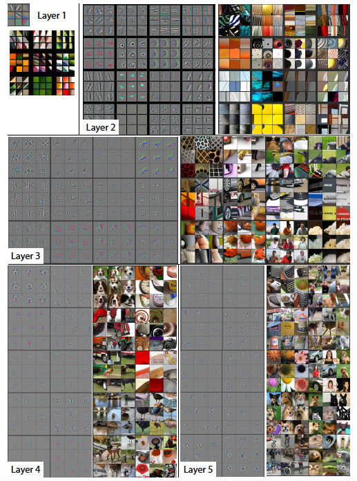
Figure 12.29: Using DeConvNets to Identify Maximally Activating Patches

We now describe the application of these ideas to generating Maximally Activating Patches using the DeConvNet algorithm, which proceeds as follows:

Start with a fully trained ConvNet model (such as on ImageNet) and present it with an input image. Do a forward pass through the model and compute all the activations.
To examine a given avtivation, set all the other activations in the Activation Map to zero and pass this map as input to the DeConvNet network.
Propagate the signal backwards using the DeConvNet propagation rules described above, until the pixel space is reached.

The reconstructed image obtained by using this procedure is shown for activations in Layers 1 to 5 in Figure 12.29. For each layer, the images on the LHS show the actual reconstruction, while the corresponding images on the RHS are portions of the input image that were identified by the reconstruction. Note that the nine largest activations were chosen in each of the Activation Maps. We can draw the following conclusions from these images:

The reconstructed image resembles a small piece of the original input image, with the shapes in the input weighted according to their contribution to the neuron whose activation was propagated back.
All the neurons in a single Activation Map seem to get activated by similar shapes, and this shape varies with the Activation Map. This property is stronger in the higher layers.
As we go up the layers, the activations get triggered by more and more complex shapes and objects.

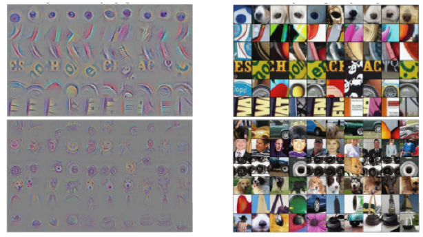
Figure 12.30: Using Guided Backpropagation to Identify Maximally Activating Patches

A similar procedure can be carried out using the Guided Backpropagation procedure, and the results for Convolutional Layers 6 and 9 are shown in Figure 12.30 (with the recosnstructed image on the LHS and the corresponding patch from the actual image on the RHS). This figure shows that the reconstructed image quality is better with Guided Backpropagation.

12.9.4 Generating Images

Generating images using ConvNets is one of the most exciting areas in Deep Learning, and as a field is still undergoing rapid development. There are several ways in which ConvNets are being used to generate images, and in this section we explore a few of them:

Generating images that maximally activate a neuron
Images generated using Google’s Deep Dream algorithm
Generating images by Feature Inversion

One of the realizations that we have to come based the image generation work, is that Neural Network models trained using Supervised Learning contain a lot of detailed information about the objects as well as other parts of the image, which is enough to actually generate images of these objects. Previously it was thought that Supervised Learning models incorporated only very basic high level information about objects, which was just sufficient to be able to recognize them. It is also possible to generate images using ConvNets with the help of Unsupervised Learning techniques such as Generative Adversarial Networks (GANs) and PixelCNN, but these are not covered in this chapter.

12.9.4.1 Generating Images that Maximally Activate a Neuron

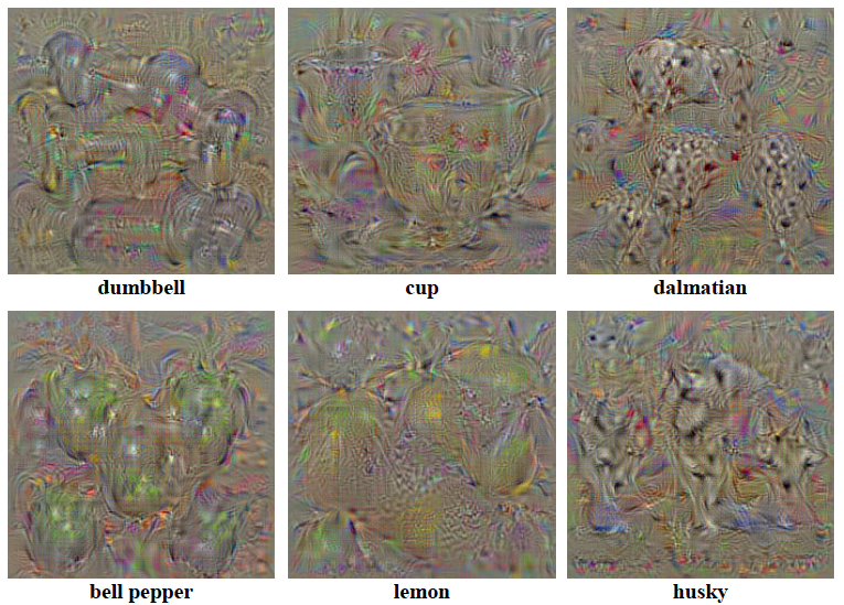
Figure 12.31: Input Images that Maximally Activate a Logit Neuron

Start with a fully trained ConvNet, and keep its weights fixed during this procedure. Solve the following maximization problem: Find an image \(I\) that maximizes the following Loss Function \[ \mathcal L = S_c(I) - \lambda ||I||^2_2 \] In this equation, the \(S_c(I)\) is the Score Function for the \(c^{th}\) class, and is computed by doing a forward pass through the ConvNet. The second term is added for doing Regularization, with \(\lambda\) as the Regularization Parameter. It had been experimentally observed that without the Regularization Term, the optimization procedure results in an image that looks like white noise.

The following algorithm isused to do the optimization:

Start with a trained ConvNet (trained on zero centered image data) and fix the value of its weights. Initialize the image pixel values \(x_{ijk}\) to zero.
Repeat Steps 3 to 5 until a Stopping Condition is satisfied
Do a forward pass through the network and compute the Score Function \(S_c(I)\) and Loss Function \(\mathcal L\).
Starting with the gradient \(\frac{\partial\mathcal L}{S_c}\), use the Backprop algorithm to compute the gradients \(\frac{\partial\mathcal L}{\partial x_{ijk}}\) of the Loss Function with respect to each of the image pixel values
Change the pixel values using the following iteration: \[ x_{ijk} \leftarrow x_{ijk} - \eta\frac{\partial\mathcal L}{\partial x_{ijk}} \]
Add the training set mean image to the final pixel values to obtain the final image.

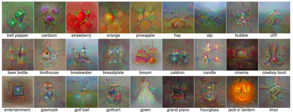
Figure 12.32: Improved Image Generation

Figure 12.31 shows the results of applying this algorithm to a ConvNet trained on the ImageNet dataset. The reader will notice the objects belonging to the category whose Score Function is being maximized, emerging at multiple places in each image, but with colors that are different than the natural coloration of the object. The reason for this is that the neurons in the later layers of the network, and especially the classification neurons, incorporate more invariance in their object recognition. Hence they recognize an object irrespective of its color or location in the image and this invariance property gets reflected in the generate images. It is possible to generate images that are more pleasing to the eye, and some of these are shown in Figure 12.32. These images were generated by making the following changes to the algorithm described above:

Incorporation of the Total Variation (TV), Gaussian Blur and Jitter regularizers into the Loss Function
Initialize the image by using the average of the images in that category from the test dataset (if an image has multiple facets, then averaging is done over one of the facets)
Use of Gaussian Blur regularization results in a blurry, but single and centered object. The optimization then proceeds by updating the center pixels more than the edge pixels to produce a final image that is sharp and is centrally located.

12.9.4.1.1 Adversarial Images

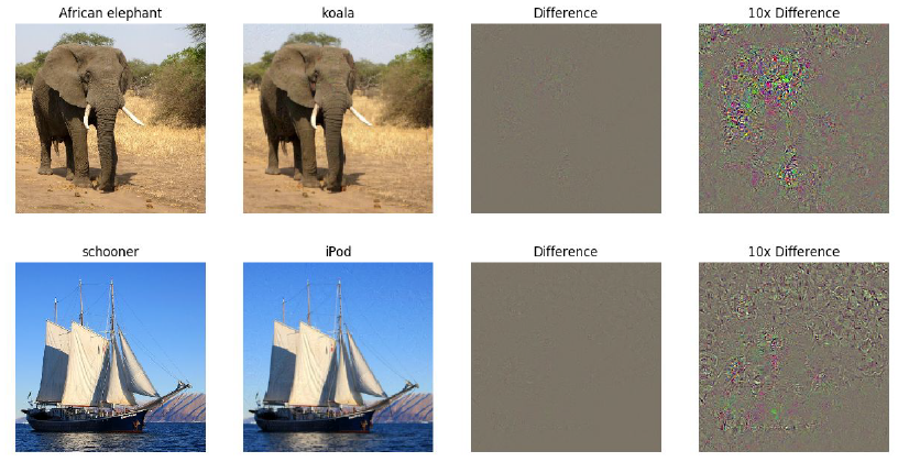
Figure 12.33: Examples of Adversarial Images

A few years ago it was discovered that ConvNets can be fooled into mis-classifying images. A couple of examples of this are shown in Figure 12.33: In the top row the first image is classified correctly as an elephant. Then this image is modified by changing some the pixels (which are shown in the last two columns), which results in the second image. These changes are not perceptible to the human eye since the second image also looks like an elephant, however when sent through a ConvNet, the system classifies it as a koala. A similar process applied to the boat in the bottom row, results in its mis-classification as an iPod. These images, which fool the ConvNet into mis-classifying them, are known as Adversarial Images.

Adversarial images can be easily created by making a slight modification to the algorithm that was presented in the prior section for generate images that maximally activate neurons. The only changes needed are the following:

Instead of initializing the input image with zeroes, we initialize it with the image whose adversarial example we wish to generate.
Choose the neuron whose activation is to be maximized, as the classification node for the adversarial image class.

We then run the maximization algorithm, and after a few iterations, the system will mis-classify the input image even though it does not appear to have changed.

Adversarial Images are an active research topic, since they constitute a significant security loophole that can perhaps be exploited.

12.9.4.2 Generating Images Using Google Deap Dream

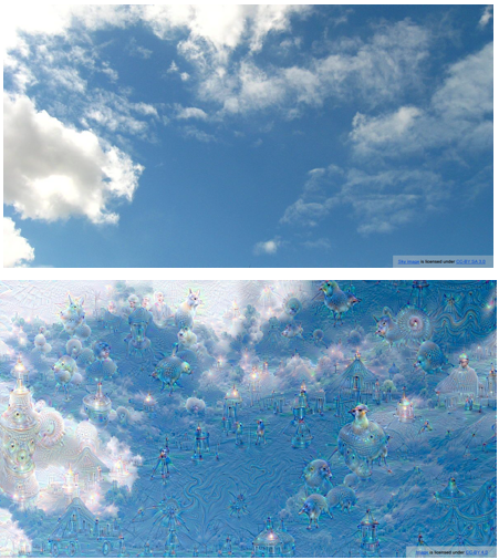
Figure 12.34: Images Generated using Deep Dream

Google Deep Dream uses the following algorithm to generate images:

Start with a trained ConvNet (trained on zero centered image data) and fix the value of its weights. Initialize the image pixel values \(x_{ijk}\) to some random image from the test dataset. In the example in Figure 12.34, the initial image was chosen to be that of clouds, shown on top part of the figure.
Repeat Steps 3 to 6 until a Stopping Condition is satisfied
Do a forward pass through the network and compute the activations at all the nodes, up until a chosen layer.
Set the gradients at each node of the chosen layer equal to the activation at that node, i.e., \[ \frac{\partial\mathcal L}{\partial z_i} = z_i \]
Using the Backprop algorithm compute the gradients \(\frac{\partial\mathcal L}{\partial x_{ijk}}\) of the Loss Function with respect to each of the image pixel values
Change the pixel values using the following iteration: \[ x_{ijk} \leftarrow x_{ijk} - \eta\frac{\partial\mathcal L}{\partial x_{ijk}} \]
Add the training set mean image to the final pixel values to obtain the final image.

In the example in Figure 12.34, the ConvNet was trained using images from the ILSVRC dataset. The top part of the figure show the input image, and after a number of iterations, the original image changes to the one shown in the bottom of figure. The Deep Dream algorithm tends to amplify random features in the original image, until they start to resemble objects that were part of the network’s original training set. Note that setting the gradient equal to the activation is equivalent to using the following Loss Function: \[ \mathcal L = {1\over 2}\sum_i z_i^2 \] where the sum is over all the activations in a given layer.

12.9.4.3 Generating Images Using Feature Inversion

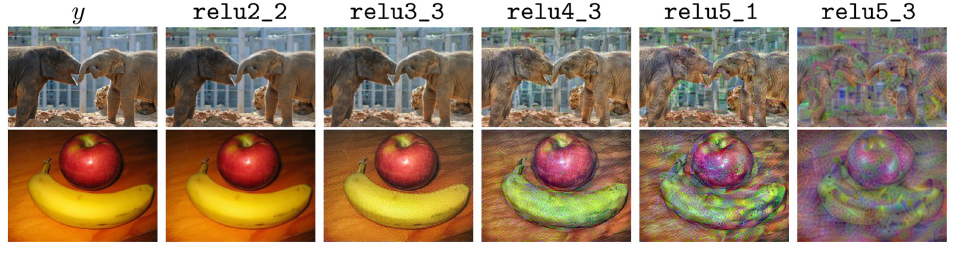
Figure 12.35: Images Generated using Feature Inversion

The image generation techniques that we have described so far, do their work by iteratively creating images that maximally activate a neuron. There is another technique, which instead of trying to maximize neuron activations, instead works by generating images whose Feature Vector is specified in advance. In order to do so, the following Loss Function is used: \[ \mathcal L = ||\Phi(X) - \Phi_0||^2 + \lambda_\alpha \mathcal R_\alpha(X) + \lambda_{V^\beta}\mathcal R_{V^\beta}(X) \] where the Regularisers \(\mathcal R_{\alpha}\) and \(\mathcal R_{V^\beta}\) are set to \[ \mathcal R_\alpha(X) = ||X||^\alpha_\alpha,\ \ {\mbox and}\ \ \mathcal R_{V^\beta}(X) = \sum_{i,j} ((x_{i,j+1} - x_{ij})^2 + (x_{i+1,j} - x_{ij})^2)^{\beta\over 2} \] In these equations \(\Phi_0\) is the Feature Vector from the test image that the algorithm is trying to match, while \(\Phi(X)\) is the Feature Vector from the current iteration of the generated image. Note that the addition of the Regularisers \(\mathcal R_{\alpha}\) and \(\mathcal R_{V^\beta}\) is critical to generating “good” images. In their absence, the algorithm will generate images whose Feature Vector minimizes the Loss Function, but which look like noise to the human eye.

The algorithm is as follows:

Start with a trained ConvNet (trained on zero centered image data) and fix the value of its weights. Initialize the image pixel \(x_{ijk}\) to some random values. The example in Figure 12.35 shows two different test images in the leftmost image in each row.
Repeat Steps 3 to 5 until a Stopping Condition is satisfied
Do a forward pass through the network and compute the activations at all the nodes, up until a chosen layer.
Compute the gradients \(\frac{\partial\mathcal L}{\partial\Phi}\) at each node of the chosen layer and use the Backprop algorithm compute the gradients \(\frac{\partial\mathcal L}{\partial x_{ijk}}\) of the Loss Function with respect to each of the image pixel values
Change the pixel values using the following iteration: \[ x_{ijk} \leftarrow x_{ijk} - \eta\frac{\partial\mathcal L}{\partial x_{ijk}} \]
Add the training set mean image to the final pixel values to obtain the final image.

The images generated by running this algorithm are shown in Figure 12.35. The notation relu2_2 is used to denote the images generated by matching feature vectors in the second layer and so on. As the figure shows, the generated images in the first few layers closely match the original test image, which implies that the ConvNet is able to store fine level details regarding the test image with a high level of fidelity. As we go to the higher layers, the image content and the overall spatial structure are preserved, but the color, texture and exact shape are not.

12.10 Implementing Conv Nets

Using Python and TensorFlow, we show how easy it is to implement a simple ConvNet for the classic MNIST problem that we have already visited in Chapter 11. The code below explains the process step-by-step. As usual, we begin by importing all the libraries we need.

%pylab inline
import keras
from keras.datasets import mnist
from keras.models import Sequential
from keras.layers import Dense, Dropout, Flatten
from keras.layers import Conv2D, MaxPooling2D
from keras import backend as K

You will see that we are using the Keras front end written by Francois Chollet to implement the model. This is a lot easier than coding up the model directly in TensorFlow. Note that we have not imported TensorFlow and it will be automatically done when invoking Keras. You should see a response from the system saying that it is using TensorFlow, which is the default. If you wish to use some other deep learning package such as Theano you will need to specifically import it. Next we load in the data for MNIST, which comes bundled with the Keras package.

data = mnist.load_data()
x_train = data[0][0]
y_train = data[0][1]
x_test = data[1][0]
y_test = data[1][1]
print(x_train.shape)
print(y_train.shape)
print(x_test.shape)
print(y_test.shape)

This produces the following output:

(60000, 28, 28)
(60000,)
(10000, 28, 28)
(10000,)

We can check what the image dimensions are.

# image dimensions
img_rows, img_cols = x_train.shape[1:3]
print(img_rows)
print(img_cols)

which gives us

28
28

For CNNs, we also need to be careful in setting up the input data and getting its shape as this is needed later when specifying the CNN structure. Here we reshape the data.

if K.image_data_format() == 'channels_first':
    x_train = x_train.reshape(x_train.shape[0], 1, img_rows, img_cols)
    x_test = x_test.reshape(x_test.shape[0], 1, img_rows, img_cols)
    input_shape = (1, img_rows, img_cols)
else:
    x_train = x_train.reshape(x_train.shape[0], img_rows, img_cols, 1)
    x_test = x_test.reshape(x_test.shape[0], img_rows, img_cols, 1)
    input_shape = (img_rows, img_cols, 1)

print(input_shape)

with the resulting shape as

(28, 28, 1)

After this, as we have done before, we normalize the input data.

x_train = x_train.astype('float32')
x_test = x_test.astype('float32')
x_train = x_train/255.0
x_test = x_test/255.0
print('x_train shape:', x_train.shape)
print(x_train.shape[0], 'train samples')
print(x_test.shape[0], 'test samples')

The checking of the shapes is shown here.

x_train shape: (60000, 28, 28, 1)
60000 train samples
10000 test samples

Recall that each digit is coded as a \(28 \times 28\) pixel frame, i.e., a set of 784 values. Each one ranges from 0 to 255, with zero signifying no ink in the pixel and 255 being the darkest color it can attain. The numerical coding of pixels is an important part of the data engineering needed for image recognition, in this case, digit recognition. For color images, this is more complex.

The next step in data engineering is to convert the tagged labels for each image into “one-hot” encoding, i.e., a matrix of ten columns, one for each digit. Each column contains a value 1 if the image is that specific digit, else it is coded as 0.

num_categories = 10
y_train = keras.utils.to_categorical(y_train, num_categories)
y_test = keras.utils.to_categorical(y_test, num_categories)
print(y_train.shape)

The output tuple is as follows and confirms the shape of the required one-hot encoding.

(60000, 10)

We are now ready to define the specific CNN we wish to deploy. The details are as follows.

model = Sequential()
model.add(Conv2D(32, kernel_size=(3, 3),
                 activation='relu',
                 input_shape=input_shape))
model.add(Conv2D(64, (3, 3), activation='relu'))
model.add(MaxPooling2D(pool_size=(2, 2)))
model.add(Dropout(0.25))
model.add(Flatten())
model.add(Dense(128, activation='relu'))
model.add(Dropout(0.5))
model.add(Dense(num_categories, activation='softmax'))

We note that the input is 2D (\(28 \times 28\)) and this is mapped into a \(3 \times 3\) kernel in the first convolutional layer. After that, the next layer is a 2D convolutional layer with 64 nodes and the \(3 \times 3\) kernel. This is followed by a max pooling layer of size \(2 \times 2\), and dropout of 25% is also applied. The 2D shape is then flattened and passed to a standard hidden layer of 128 nodes with a ReLU activation function. Then, a 50% dropout is applied. Finally, a softmax output layer generates a categorical decision to choose one of the ten possible digit categories.

As is required with TensorFlow, the model is then compiled.

model.compile(loss=keras.losses.categorical_crossentropy,
              optimizer=keras.optimizers.Adadelta(),
              metrics=['accuracy'])

The compiled model is then fit.

epochs = 5
batch_size = 128
model.fit(x_train, y_train,
          batch_size=batch_size,
          epochs=epochs,
          verbose=1,
          validation_data=(x_test, y_test))

Note that the number of epochs has been specified as just 5, which is extremely low, but this has been done to save time and for parsimony of output. Here are the run time results.

Train on 60000 samples, validate on 10000 samples
Epoch 1/5
60000/60000 [==============================] - 335s - loss: 0.3312 - acc: 0.8993 - val_loss: 0.0814 - val_acc: 0.9740
Epoch 2/5
60000/60000 [==============================] - 446s - loss: 0.1178 - acc: 0.9653 - val_loss: 0.0541 - val_acc: 0.9820
Epoch 3/5
60000/60000 [==============================] - 429s - loss: 0.0892 - acc: 0.9740 - val_loss: 0.0482 - val_acc: 0.9844
Epoch 4/5
60000/60000 [==============================] - 447s - loss: 0.0746 - acc: 0.9777 - val_loss: 0.0395 - val_acc: 0.9855
Epoch 5/5
60000/60000 [==============================] - 469s - loss: 0.0656 - acc: 0.9805 - val_loss: 0.0365 - val_acc: 0.9876

This was run on an extremely low-end laptop, and not on GPUs, as is often the case. Each epoch takes about 6-8 minutes and the entire model fitting therefore takes more than a half hour. Notice how much slower fitting a CNN is to a standard feedforward neural net, which usually takes less than a minute of run time. You can see how the model slowly increases in accuracy with each epoch. Eventually, this model achieves close to 99% accuracy, as we see next.

score = model.evaluate(x_test, y_test, verbose=0)
print('Test loss:', score[0])
print('Test accuracy:', score[1])

with accuracy

Test loss: 0.0365297323162
Test accuracy: 0.9876

References

Hubel, D. H., and T. N. Wiesel. 1959. “Receptive Fields of Single Neurones in the Cat’s Striate Cortex.” The Journal of Physiology 148 (3): 574–91. doi:10.1113/jphysiol.1959.sp006308.

Hubel, D. 1962. “Receptive Fields, Binocular Interaction and Functional Architecture in the Cat’s Visual Cortex.” The Journal of Physiology 160 (1): 106–54. doi:10.1113/jphysiol.1962.sp006837.

Hubel, David H., and Torsten N. Wiesel. 1968. “Receptive Fields and Functional Architecture of Monkey Striate Cortex.” Journal of Physiology (London) 195: 215–43.

Fukushima, Kunihiko. 1975. “Cognitron: A Self-Organizing Multilayered Neural Network.” Biological Cybernetics 20 (3): 121–36. doi:10.1007/BF00342633.

Fukushima, Kunihiko. 1980. “Neocognitron: A Self-Organizing Neural Network Model for a Mechanism of Pattern Recognition Unaffected by Shift in Position.” Biological Cybernetics 36 (4): 193–202. doi:10.1007/BF00344251.

LeCun, Yann, Léon Bottou, Yoshua Bengio, and Patrick Haffner. 1998. “Gradient-Based Learning Applied to Document Recognition.” In Proceedings of the Ieee, 2278–2324.

Russakovsky, Olga, Jia Deng, Hao Su, Jonathan Krause, Sanjeev Satheesh, Sean Ma, Zhiheng Huang, et al. 2015. “ImageNet Large Scale Visual Recognition Challenge.” International Journal of Computer Vision (IJCV) 115 (3): 211–52. doi:10.1007/s11263-015-0816-y.

Krizhevsky, Alex, Ilya Sutskever, and Geoffrey E. Hinton. 2012. “ImageNet Classification with Deep Convolutional Neural Networks.” In Proceedings of the 25th International Conference on Neural Information Processing Systems - Volume 1, 1097–1105. NIPS’12. Lake Tahoe, Nevada. http://dl.acm.org/citation.cfm?id=2999134.2999257.

Zeiler, Matthew D., and Rob Fergus. 2013. “Visualizing and Understanding Convolutional Networks.” CoRR abs/1311.2901. http://arxiv.org/abs/1311.2901.

Simonyan, Karen, and Andrew Zisserman. 2014. “Very Deep Convolutional Networks for Large-Scale Image Recognition.” CoRR abs/1409.1556. http://arxiv.org/abs/1409.1556.

Szegedy, Christian, Sergey Ioffe, and Vincent Vanhoucke. 2016. “Inception-V4, Inception-Resnet and the Impact of Residual Connections on Learning.” CoRR abs/1602.07261. http://arxiv.org/abs/1602.07261.

He, Kaiming, Xiangyu Zhang, Shaoqing Ren, and Jian Sun. 2015a. “Deep Residual Learning for Image Recognition.” CoRR abs/1512.03385. http://arxiv.org/abs/1512.03385.