Chapter 4 Linear Learning Models
4.1 Logistic Regression
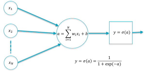
Figure 4.1: A Linear Model for Classifying into 2 Categories
The subject of this chapter are Linear Neural models used for classification, which also go by the name Logistic Regression. These models serve as the building block for more sophisticated DLN models, all of whom use a Logistic Regression layer for their final classification stage.
Using the notation from the previous chapter, the functional form of the simplest linear model with single node in the Output Layer (corresponding to \(K=2\)) is given by
\[\begin{equation} a = \sum_{i=1}^N w_i x_i + b \tag{4.1} \end{equation}\]In this equation \((w_1,...,w_N)\) are called weights and \(b\) is known as the bias (see Figure 4.1). As the reader can readily see, \(a\) can not function as the output of a classification system, since we cannot ensure that \(0 \le a\le 1\). In order to satisfy this requirement we add a function called the sigmoid to the system (see Figure 4.2). The sigmoid function is also referred to as the “squashing function” since it maps the entire real axis into the finite interval \([0, 1]\). The resulting output \(y\) satisfies the condition \(0\le y\le 1\) and hence is a suitable output for the Logistic Regression system.
\[ y = \sigma(a) = \frac{1}{1+\exp(-a)} \]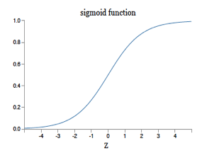
Figure 4.2: The Sigmoid Function
We can do classification using this model by using the following criteria: If \(y\ge 0.5\), then the model predicts that input to be in class 1, or else in class 2. Note that the condition \(y\ge 0.5\) is equivalent to the condition \[ a = \sum_{i=1}^N w_i x_i + b \ge 0 \] so that input points on one side of the hyperplane \(\sum_{i=1}^N w_i x_i + b\) are categorized in class 1, and those on the other side are categorized in class 2. This leads to the question: Why not use \(a\) to do the classification, thus avoidng the extra step of computing \(y\). If we use the criteria \(y\ge 0.5\) to do the classification, then indeed there is no difference in whether we choose to use \(y\) or \(a\). However if we change the classification criteria to the following: Compute \(y\) and use it to generate a Random Number such that the probability of the input being in class 1 is \(y\), and similarly for class 2. With this criteria, there is a finite chance that the predicted class is \(2\), even though \(y\ge 0.5\) (especially if \(y\) is close to \(0.5\)). This means that input points that are close to the hyperplane \(a = \sum_{i=1}^N w_i x_i + b\) have an equal chance of being classified in either Class 1 or Class 2. This distinction is important, since it enables the Logistic Regression model to use probabilistic inference and do classification even in cases in which the two classes are not strictly linearly separated. The interpretation of the Linear Model as a hyperplane also explains the need for the bias parameter \(b\), since in the absence of \(b\), all hyperplanes would be constrained to pass through the origin, which obviously limits their modeling power.
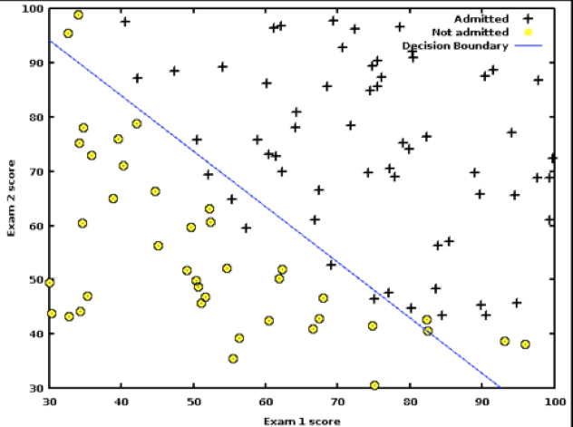
Figure 4.3: The Linear Separator in Logistic Regression
Figure 4.3 shows the results of applying Logistic Regression in the two dimensional case to a test dataset. As we noted earlier, point that are close to the linear separator may get classified in either of the two classes due to the statistical nature of the algorithm.
Now that we have obtained the structural form for our classification system for the special case \(K=2\), the next step is to estimate the model parameters \(b, w_i, i=1,...,N\) from the training data. From the discussion in the prior chapter, this can be done by choosing the parameters so that they minimize the Cross Entropy Loss Function. Given that \((X{(m)},T{(m)}),m=1,...,M\) is the training sequence, the Loss Function is defined as:
\[ L = -{1\over M}\sum_{m=1}^M t{(m)} \log y{(m)} + (1-t{(m)}) \log(1-y{(m)}) \] where the output \(y{(m)}\) in response to the \(m^{th}\) input vector \(X{(m)}\) is given by
\[ y{(m)} = \sigma(a{(m)})\ \ where\ \ a{(m)} = \left(\sum_{i=1}^N w_i x_i{(m)} + b \right), \ \ 1\le m\le M \] Even for this simple model there is no closed form solution for determining the values of \((W,b)\) that minimize \(L\), so we resort to the use of the Gradient Descent algorithm:
\[ w_i \leftarrow w_i - \eta \frac{\partial L}{\partial w_i},\ \ 1\le i\le N\ and\ b\leftarrow b - \eta \frac{\partial L}{\partial b} \] where \(\eta\) is a constant called the Learning Rate. There are various ways in which the iteration shown above can be improved and is discussed in detail in Chapter 7. In order to proceed we need to compute the gradients \(\frac{\partial L}{\partial w_i}\) and \(\frac{\partial L}{\partial b}\).
The Loss Function \(\mathcal L\) for a single sample of the training dataset is given by: \[ \mathcal L = -(t\log y + (1-t)\log (1-y)) \] Using the Chain Rule of Derivatives, \[ \frac{\partial \mathcal L}{\partial w_i} = \frac{\partial \mathcal L}{\partial y}\frac{\partial y}{\partial a}\frac{\partial a}{\partial w_i} \] Note that \[ \frac{\partial \mathcal L}{\partial y} = \frac{y-t}{y(1-y)},\ \ \frac{\partial y}{\partial a} = y(1-y)\ \ and\ \ \frac{\partial a}{\partial w_i} = x_i \] which results in \[ \frac{\partial \mathcal L}{\partial w_i} = x_i(y-t),\ 1\le i\le N \] We can now write down the expression for the derivative of the Loss Function \(L\) for the entire training dataset:
\[\begin{equation} \frac{\partial L}{\partial w_i} = -{1\over M}\sum_{m=1}^M x_i(m)(y{(m)}-t{(m)}),\ 1\le i\le N \tag{4.2} \end{equation}\]Using equation (4.2), the following iterative algorithm can be used to train the model:
Gradient Descent Algorithm
Initialize all the weights \(w_i, 1\le i\le N\) and the bias term \(b\) to zero.
- In response to the training sequence \(X{(m)}, 1\le m\le M\), compute the model predictions \(y(m), 1\le m\le M\) (using the latest values of the parameters \((W,b)\)): \[ y(m) = \sigma\left(\sum_{i=1}^N w_i x_i{(m)} + b \right), \ \ 1\le m\le M \]
Change the model parameters according to the formulae
\[ b \leftarrow b - {\eta\over M} \sum_{m=1}^M (y{(m)}-t{(m)}) \]
- Compute the Loss Function \(L\) over the Validation Dataset given by \[ L = -{1\over V}\sum_{m=1}^V t{(m)} \ln y{(m)} + (1-t{(m)} \ln(1-y{(m)}) \] where \(V\) is the number of samples in the Validation Dataset. If \(L\) drops below some threshold, then stop. Otherwise go back to Step 2.
An alternative to using the Loss Function as a stopping criteria, is to use a performance measure called Accuracy. This is defined as the percentage of correct predictions on the Validation Dataset, so that, the Accuracy \(A\) is given by \[ A = \frac{ \sum_{m=1}^V 1_{y(m)=t(m)}} {V} \] If the value of \(A\) exceeds some threshold, terminate the algorithm.
The Gradient Descent Algorithm is our first encounter with training or learning algorithms in this monograph. The mathematical setup and general procedure that we used in this algorithm holds true for more complex models. Step 2 of the algorithm in which the output of the model is computed is known as the Forward Pass. Step 3 of the model in which the gradients are computed and then used to update the model parameters, is known as the Backward Pass. This model (and all other DLN models) proceeds by repeated cycles of Forward and Backward Passes, until the stopping condition is satisfied.
In ML algorithms, an epoch is defined as the time required to do a single pass through all the elements in the training dataset. In the algorithm described above, note that model parameters are updated only once per epoch. In practice, this considerably slows down the speed of convergence, especially for large training datasets. We now present a modification to the algorithm, called Stochastic Gradient Descent (SGD), which updates the parameters more frequently, indeed after processing each element in the training dataset. The key to SGD is the observation that the parameter update equation can be written as:
\[\begin{equation} w_i \leftarrow w_i - \eta x_i(m)(y{(m)}-t{(m)}),\ 1\le i\le N \tag{4.4} \end{equation}\]Hence for input vector \(X(m)\), we compute the corresponding output \(y(m)\), and then use the above equation to immediately change the model parameters, and then repeat the process with the next input. This considerably speeds up the algorithm, and thus the learning process. Effectively by doing this, we are using noisy estimates of the gradient to do the iteration, which causes the convergence to be not as smooth as with Gradient Descent (see Figure 4.4). However it has been observed that the noise introduced to SGD also has the benefit of helping the algorithm avoid getting stuck in non-optimal minima, as well as escape from saddle point quickly.
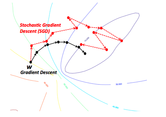
Figure 4.4: Stochastic Gradient Descent
Stochastic Gradient Descent Algorithm (SGD)
Initialize all the weights \(w_i, 1\le i\le N\) and the bias term \(b\) to zero.
For \(m = 1,...,M\) repeat the following steps (a) - (c):
- For the input vector \(X{(m)}\), compute the model prediction \(y(m)\) given by \[ y(m) = \sigma\left(\sum_{i=1}^N w_i x_i{(m)} + b \right) \]
- Change the model weights according to the formula
\[ w_i \leftarrow w_i - \eta x_i(m)(y{(m)}-t{(m)}),\ 1\le i\le N \]
\[ b \leftarrow b - \eta (y{(m)}-t{(m)}) \]
- Increment \(m\) by one and go back to step \((a)\).
- Compute the Loss Function \(L\) over the Validation Dataset given by \[ L = -{1\over V}\sum_{m=1}^V t{(m)} \log y{(m)} + (1-t{(m)} \log(1-y{(m)}) \] If \(L\) has dropped below some threshold, then stop. Otherwise go back to Step 2.
Note that in the SGD algorithm we update the parameter values after processing each element in the training dataset, but we check the stopping condition only once per epoch.
There is a third way of solving the optmization problem, which is midway between the two extremes of Gradient Descent and Stochastic Gradient Descent, and is known as Batch Stochastic Gradient Descent (B-SGD). This is based on the following parameter update rule: \[ w_j \leftarrow w_j - {\eta\over B} \sum_{b=1}^B x_i(b)(y{(b)}-t{(b)}) \] This algorithm works by dividing up the training dataset into batches of size \(B\), and then updates the parameters only once per batch. By varying the batch size, we can trade-off the smoothness of the convergence algorithm with the speed of convergence.
Batch Stochastic Gradient Descent Algorithm (B-SGD)
Initialize all the weights \(w_i, 1\le i\le N\) and the bias term \(b\) to zero.
For \(r = 0,...,{M\over B}-1\) repeat the following steps (a) - (c):
- For the training inputs \(X_i(m), rB\le i\le (r+1)B\), compute the model predictions \(y(m)\) given by
\[ y(m) = \sigma\left(\sum_{i=1}^N w_i x_i{(m)} + b \right) \]
- Change the model weights according to the formula
\[ w_j \leftarrow w_j - {\eta\over B} \sum_{m=rB}^{(r+1)B} x_i(m)(y{(m)}-t{(m)}),\ 1\le j\le N \] \[ b \leftarrow b - {\eta\over B} \sum_{m=rB}^{(r+1)B}(y{(m)}-t{(m)}) \]
- Increment \(r\) by one and go back to step \((a)\).
- Compute the Loss Function \(L\) over the Validation Dataset given by \[ L = -{1\over V}\sum_{m=1}^V t{(m)} \ln y{(m)} + (1-t{(m)} \ln(1-y{(m)}) \] If \(L\) has dropped below some threshold, then stop. Otherwise go back to Step 2.
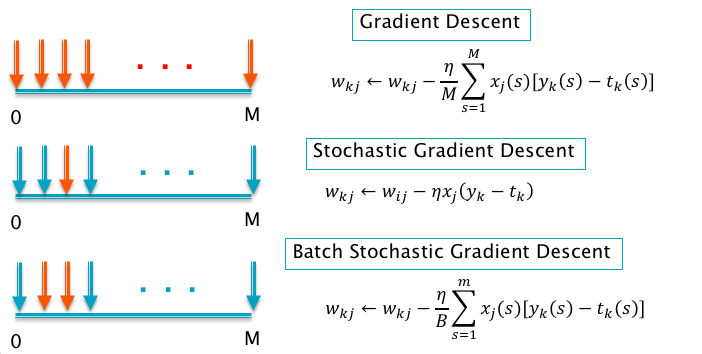
Figure 4.5: Comparison of Gradient Descent Algorithms
Figure 4.5 gives a summary of the three Gradient Descent algorithms types, with the red arrows representing the number of input samples that are used in the computation of a single update of the model parameters.
4.2 Multiclass Logistic Regression
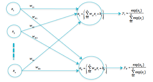
Figure 4.6: The Multiclass Logistic Regression
If the input can belong to one of \(K\) categories, then the Logistic Regression model can be expanded to accommodate this, as shown in Figure 4.6. Define the quantities \(a_k\) by
\[ a_k = \sum_{i=1}^N w_{ki} x_i + b_k, \quad 1 \leq k \leq K \] These quantities are referred to as logits in Machine Learning literature, and are defined as the outputs of the final layer of neurons. They are also sometimes referred to as “Scoring Functions”, since a higher score for a class means that it stands a greater chance of being the selected category.
We need to convert these logits into output probabilities \(y_k\). Note that the sigmoid function cannot be used for this, since in that case the condition \(\sum_{k=1}^K y_k = 1\) is not guaranteed to be satisfied. Instead the probabilities are generated using the following equation:
\[ y_k = \frac{\exp(a_k)}{\sum_{i=1}^K \exp(a_i)}, \quad 1 \leq k \leq K \] which is called the Normalized Exponential or Softmax function and is a multiclass generalization of the sigmoid. Indeed for the case \(K = 2\) it is easy to show that softmax and the sigmoid result in identical outputs.
The Loss Function for this model can be written as
\[ L = -{1\over M}\sum_{m=1}^M \sum_{k=1}^K t_k(m)\log y_k(m) = {1\over M}\sum_{m=1}^M \mathcal L(m) \] where \[ \mathcal L(m) = -\sum_{k=1}^K t_k(m)\log y_k(m) \]
In order to train the model using Gradient Descent, we need to compute \(\frac{\partial \mathcal L}{\partial w_{ki}}\) and \(\frac{\partial \mathcal L}{\partial b_{k}}\). Using the Chain Rule of derivatives \[ \frac{\partial \mathcal L}{\partial w_{ki}} = \frac{\partial \mathcal L}{\partial a_{k}}\frac{\partial a_k}{\partial w_{ki}} \] Note that \(\frac{\partial a_k}{\partial w_{ki}} = x_i\) while \(\frac{\partial \mathcal L}{\partial a_{k}}\) can be written as \[ \frac{\partial \mathcal L}{\partial a_{k}} = \sum_{j=1}^K \frac{\partial \mathcal L}{\partial y_{j}} \frac{\partial y_j}{\partial a_{k}} \] In order to justify this equation, note that the logit \(a_k\) influences the Loss Function through all of the outputs \(y_j, 1\le j\le K\), due to the form of the softmax equation. Note that \[ \frac{\partial \mathcal L}{\partial y_{j}} = -\frac{t_j}{y_j} \] while it is not difficult to show that \[ \frac{\partial y_j}{\partial a_{j}} = y_j(1-y_j) \] and \[ \frac{\partial y_j}{\partial a_{k}} = -y_jy_k\ \ for\ \ j\ne k \] It follows that \[ \frac{\partial \mathcal L}{\partial a_{k}} = -\frac{t_k}{y_k} y_k(1-y_k) - \sum_{j\ne k}\frac{t_k}{y_j}(-y_jy_k) = -(t_k - t_ky_k-\sum_{j\ne k}t_jy_k) = -(t_k-\sum_{j=1}^K t_jy_k) = y_k-t_k \] Putting all these equations together, it follows that \[ \frac{\partial \mathcal L}{\partial w_{ki}} = x_i(y_k - t_k) \] Similarly it can be shown that \[ \frac{\partial \mathcal L}{\partial b_{k}} = (y_k - t_k) \] Using these expressions, we end up with the following Gradient Descent Training Algorithm for Logistic Regression systems with \(K\) output categories:
Gradient Descent Algorithm
Initialize all the weights \(w_{ki}, 1\le k\le K, 1\le i\le N\) and the bias terms \(b_k, 1\le k\le K\) to zero.
- In response to the training sequence \(X{(m)}, 1\le m\le M\), compute the model predictions \(y_k(m), 1\le k\le K, 1\le m\le M\) (using the latest values of the parameters \((W,b)\)): \[ y_k(m) = \sigma\left(\sum_{i=1}^N w_{ki} x_i{(m)} + b_k \right),\ \ 1\le k\le K,\ \ 1\le m\le M \]
Change the model parameters according to the formulae
\[ w_{ki} \leftarrow w_{ki} - {\eta\over M} \sum_{m=1}^M x_i(m)(y_k{(m)}-t_k{(m)}),\ 1\le k\le K,\ 1\le i\le N \]
\[ b_k \leftarrow b_k - {\eta\over M} \sum_{m=1}^M (y_k{(m)}-t_k{(m)}), \ \ 1\le k\le K \]
- Compute the Loss Function \(L\) over the Validation Dataset given by \[ L = -{1\over V}\sum_{m=1}^V\sum_{k=1}^K t_k{(m)} \log y_k{(m)} \] where \(V\) is the number of samples in the Validation Dataset. If \(L\) drops below some threshold, then stop. Otherwise go back to Step 2.
4.3 Image Classification Using Linear Models
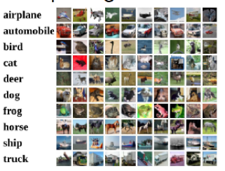
Figure 4.7: The CIFAR-10 Image Dataset
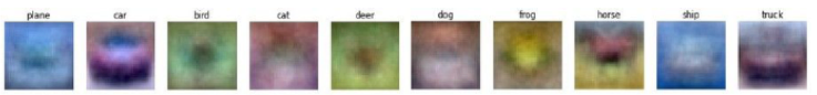
Figure 4.8: Templates Created from Linear Classifier Weights
A Linear Classifier can be interpreted as a straight line (in 2-D) or hyperplane that separates out the points belonging to the classes being categorized. There is another interpretation of Linear Classifiers which is best understood for the case when the input is an image, and this is in terms of Template Matching. We introduced the MNIST image dataset in Chapter 2, and we now introduce the CIFAR-10 image dataset which has also played an important role in the development of DLNs (see Figure 4.7). This dataset consists 50,000 training images and 10,000 test images, each of which is 32x32x3 pixels. Each image contains an object which can belong to one of ten categories, as shown in the figure.
In order to input a CIFAR-10 image into the classifier, it has to be stretched out into a vector of 3072 dimensions. It is then fed into the 10-ary classification model of the type shown in Figure 4.6. A fully trained linear model results in a classification accuracy of about 40%, which is significantly higher than the accuracy of 10% or so one would expect if we were to make a purely random choice. We can get some understanding of the way the images are being classified by examining the weight matrix \(\{w_{ki}\}, 1\le k\le 10, 1\le i\le 3072\). Recall that the logits \(a_k, 1\le k\le 10\) are defined as
\[\begin{equation} a_k = \sum_{i=1}^{3072 } w_{ki} x_i,\ \ 1\le k\le 10 \tag{4.5} \end{equation}\]where \(x_i\) represent the pixels in the image. Lets assume that the input image belongs to the category \(q\). In order to correctly classify this image, the logit \(a_q\) should be significantly larger than the other logits. How does the system accomplish this? A plausible explanation can be obtained by considering Equation (4.5) to be a form of template matching. Just as we obtained the vector \(x_i, 1\le i\le 3072\) by stretching out the image pixels, we can also reverse this process and create an image from the weight vector \(w_{qi}, 1\le i\le 3072\) that is used to compute the \(q^{th}\) logit \(a_q\). The images thus created from the weight vectors for the ten CIFAR-10 categories are shown in Figure 4.8. The reader will notice that there is a faint but distinct resemblance between these “weight generated” images and the category to which the weights belong. This can be explained by interpreting the “weight generated” images as an image template. Hence a fully trained model creates ten of these templates, one for each image category, and then it does classification by using Equation (4.5) to do template matching (it can be shown that under a norm constraint, the sum in Equation (4.5) is maximized if the vectors \(w_{.i}\) and \(x_i\) match).
The explanation that we gave in terms of template matching, points to the interpretation of the model weight parameters as a filter. This interpretation is extremely important, and serves as the inspiration for a class of DLN models called Convolutional Neural Networks (see Chapter 12).
4.4 Beyond Linear Models
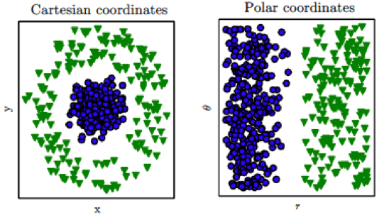
Figure 4.9: Non Linearly Separable Dataset
Note that Linear Models work well only in cases in which the data categories are approximately linearly separable. In the 2-dimensional case this corresponds to drawing a straight line that separates out most of the points in the two categories. However there are cases in which this assumption does not hold, an example of which is shown in the diagram on the LHS of Figure 4.9. Some of these cases can be solved by finding new representations for the input data in which the linear separability property holds. For example if we change the co-ordinates in Figure 4.9 from Cartesian to Polar, then the two classes become linearly separable. The change in representation for the general case (for K = 2) is shown in Figure 4.10, so that the output of this network is given by: \[ y = \sigma(\sum_{i=1}^N w_i f_i(x_1,...,x_N) + b) \]
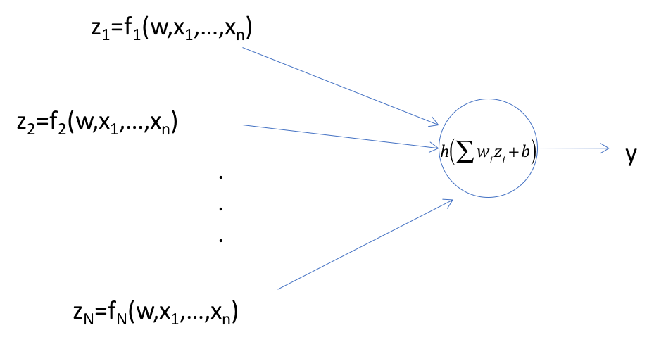
Figure 4.10: Logistic Regression with Feature Extraction
Before the discovery of DLNs, a lot of the research in the classification area was focused on pre-processing the input values and discovering appropriate functions \(f_i\) (known as Feature Extractors) which could then be fed into the Logistic Regression network. The Feature Extractor selection involves a deep analysis of the original input to discover functions that can transform the input data in a way that makes it amenable to classification using a simple linear system.
DLNs have done away with the intermediate step of manual feature set selection. As explained in the next chapter, DLNs automatically learn the appropriate representation from the available training data, using an algorithm that is a generalization of the one we discussed for Logistic Regression.