Chapter 1 Introduction

There is a lot of excitement surrounding the fields of Neural Networks (NN) and Deep Learning (DL), due to numerous well-publicized successes that these systems have achieved in the last few years. The objective of this monograph is to provide a concise survey of this fast developing field, with special emphasis on more recent developments. We will use the nomencalture Deep Learning Networks (DLN) for Neural Networks that use Deep Learning algorithms.

DLNs form a subfield within the broader area of Machine Learning (ML). ML systems are defined as those that are able to train (or program) themselves, either by using a set of labeled training data (called Supervised Learning), or even in the absence of training data (called Un-Supervised Learning). In addition there is a related field called Reinforcement Learning in which algorithms are trained not by training examples, but by using a sequence of control actions and rewards. Even though ML systems are trained on a finite set of training data, their usefulness arises from the fact that they are able to generalize from these and process data that they have not seen before.

Most of the recent breakthroughs in DLNs have been in Supervised Learning systems, which are now being widely used in numerous applications in industrial and consumer settings, some of these are enumerated below:

• Image Recognition and Object Detection: DLNs enable the detection and classification of objects in images into one of more than thousand different categories. This has hundreds of applications ranging from diagnosis in medical imaging to security related image analysis.

• Speech Transcription: DLN systems are used to transcribe speech into text with a high level of accuracy. Advances in this area have enabled products such as Amazon’s Alexa and Apple’s Siri.

• Machine Translation: Large scale translation systems such as the one deployed by Google, have switched over to using DLN algorithms (Sutskever, Vinyals, and Le 2014).

• Self Driving Cars: DLN systems are enabling Self Driving Cars as well as advances in Robotics.

Image Recognition belongs to the class of applications that involve classification of the input into one of several categories. The Speech Transcription and Machine Translation applications involve not just recognition of the input pattern, but also the generation of patterns as part of the output (so called Generative Models). The Self Driving car application uses images from its camera for its input, but the output now consists of Control Actions, such as steering and braking.

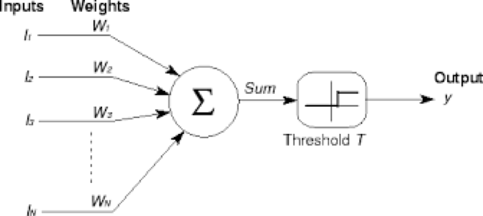
Figure 1.1: McCullough Pitts neuron

NNs have existed since the 1940s, when they were first proposed by McCulloch and Pitts (1943) as a model for biological neurons. As shown in Figure 1.1, this model consisted of a set of inputs, each of which was multiplied by a weight and then summed over. If the sum exceeded a threshold, then the network outputted a \(+1\), and \(-1\) otherwise. These was a simple model in which weights were fixed and the output was restricted to \(\{+1,-1\}\). The idea of Hebbian learning was discovered around the same time, in which learning was accomplished by changing the weights. The idea of NNs was then taken up Rosenblatt in the 1950s and 60s, see Rosenblatt (1958) and Rosenblatt (1962), who combined the ideas of the McCullough-Pitts neuron with that of Hebbian learning, and referred to his model as a Perceptron.

Perceptrons achieved some early successes, but ran into problems when researchers tried to use them for more sophisticated classification problems. In particular, the Perceptron learning algorithm fails to converge in cases in which the data is not strictly linearly separable. These problems with Perceptrons, along with the publication of a book on this topic by Minsky and Papert (1969), where these issues were highlighted, led to a drop in academic interest in NNs, which persisted until the early 80s. There were two advances that moved the field beyond Perceptrons and led to the modern idea of DLNs:

• The incorporation of techniques from Statistical Estimation and Inference into ML: A critical step was the replacement of deterministic 0-1 classification by probabilistic classifiers based on Maximum Likelihood estimation. This ensured that the learning algorithms converged even for cases in which the classes were not strictly linearly separable.

• The discovery of the Backprop algorithm: This was a critical advance that enabled the training of large multi-layer DLNs. Even today Backprop serves as the main learning algorithm for all DLN models.

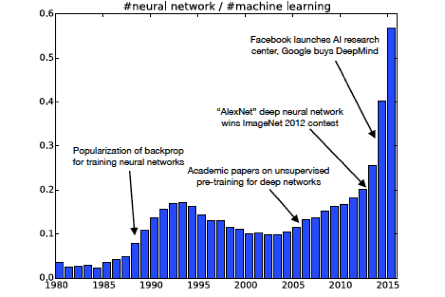
Figure 1.2: Number of DLN research reports

As shown in Figure 1.2, these discoveries resulted in renewed interest in NNs from the mid-80s onwards, which persisted till the mid-90s. Around that time, attempts to use the Backprop algorithm to train very large NNs led to an issue known as the Vanishing Gradient problem, discussed in Chapter 7. As of a result of this problem, Backprop based systems stopped learning after some number of iterations, i.e., their weights stopped adapting to new training data. At the same time, a new ML algorithm called Support Vector Machine (SVM) was discovered that worked much better in NNs for large classification problems. As a result of this, interest in DLNs once again dipped in the late 90s and didn’t recover until recently.

As Figure 1.2 shows, growth in DLN related research has exploded in the last 8-10 years, which is often referred to as the “Neural Networks Renaissance”. Several factors have contributed to this, among them:

• The increase in CPU processing power and use of specialized CPUs optimized for NN processing: Researchers discovered that processors built for Graphics Processing, or GPUs, were very effective in doing DLN computations as well. A new generation of processors built especially for DLN processing is also coming to market.

• The application of Big Data techniques to the problem: Software architectures such as Hadoop, which enable large scale and massive parallelism, have been applied to DLN processing, resulting in considerable speedup in model training and execution. In combination with the use of GPUs, this has enabled DLNs containing millions of nodes which are capable to solving very sophisticated problems.

• The availability of crowd sourced massive labeled data-sets that can be used for training large DLNs. This has been mainly due to the rise of the Internet and its database of millions of images.

• Algorithmic and Architectural Advances: Among the algorithmic advances are (a) Techniques to solve the Vanishing Gradient problem for large DLNs Hahnloser et al. (2000), Nair and Hinton (2010), and (b) Techniques to improve the generalization ability of DLNs Srivastava (2013). Among the architectural advances are the discovery of new DLN configurations such as Convolutional Neural Networks (CNN) and Recurrent Neural Networks (RNN). CNNs are well suited for processing images, while RNNs are designed for learning patterns in sequences of data, such as language or video streams.

1.1 Why are DLNs so Effective

DLNs differentiate themselves by their effectiveness in solving problems in which the input data has hundreds of thousands of dimensions. A good examples of such an input is a color image, for example consider an image which consists of three layers (RGB) of 224 X 224 pixels. The total number of pixels in such an image is 150,528, any of which may carry useful information about the it. If we want to process this image and extract useful information from it (such as, classify all objects or describe the scene), this problem is very difficult to solve using non-DLN systems. How are DLNs able to solve this problem? In order to aswer this question consider Figure 1.3. As the figure shows, the DLN can be considered to be a function that transforms the input representation, which has 150K dimensions, to an output representation that has 4K dimensions. This output representation has useful structural properties and in particular captures semantic information reagrding the input.

An example of a structural property, that enables the system to classify the input image into one of several categories, is the following: If we plot the coordinates of the output representation, then it can be verified that the points representing images that are similar to each other, also tend to cluster together. An example of this is seen in Figure 1.4, in which we plot the transformed representations for a dataset called MNIST. This dataset consists of 784-dimensional handwritten images of the digits from 0 to 9 (see Figure 2.1).The figure shows the 4096 dimensional output representations corresponding to the images of digits after they have passed through a DLN. These points are actually projected from 4096-dimensional to 2-dimesional space, using a technique called t-SNE in order to aid human comprehension. Note that the representations of a particular digit are clustered together. This clustering is a very useful property to have, since it enables the subsequent classification of these points into categories by using a simple linear classifier. The key point to note is that the clustered points now carry semantic information about the input image.

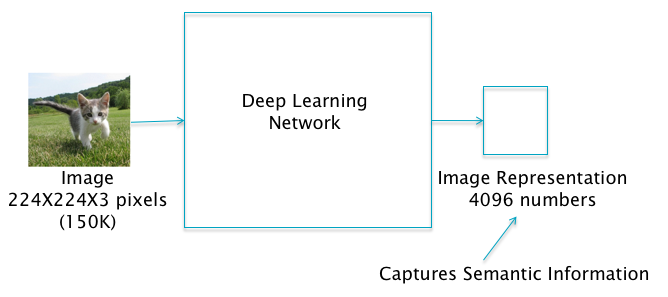
Figure 1.3: Image Representation Transform

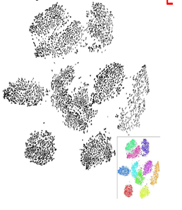
Figure 1.4: MNIST Data after Transform

The process described in the previous paragraph is called Representation Learning, since the DLN transforms the input representation of each image (in terms of RGB pixels) to an output representation that is more suitable for doing tasks such as classification. Before the advent of DLN systems, tasks such as image classification were carried out with the designer required to come up with a suitable output representation herself. This was a fairly time consuming job requiring a lot of expertise, and typically took several years to come up with a good representation for a particular class of problems. DLN systems have automated this process, such that the system learns the best output representation for a problem on its own, by using the training dataset.

Another way to understand the process by which DLN systems create representations and do classification for images in shown in Figure 1.5. The figure shows a DLN with 4 so-called Hidden Layers followed by the final Output Layer which classifies the image into one of three categories (these layers are formally defined in the next chapter). The first Hidden Layer acts upon the raw pixels and acts as a detector for edges in the image, such that each node in this layer is reponsible for detecting edges in different orientations. Note that edges can be detected fairly easily by comparing the brightness level of neighboring pixels. The second Hidden Layer acts on the output of the First Hidden Layer and detects features that are composed from putting together multiple edges together, such as corners and contours. The third Hidden Layer further builds on this, and detects object parts that composed from corners and contours. This functions as the output representation of the Input Image, and the final Layer (which is also called the Logit Layer) acts on this representation to put together the whole object, and thus carry out the classification task with a linear classifier. As this description shows, each successive layer in a DLN system, builds on the layer imemediately preceding it and thus creates representations for objects in an hierarchical fashion, by starting with the detection of simple features and then going on to more complex ones.

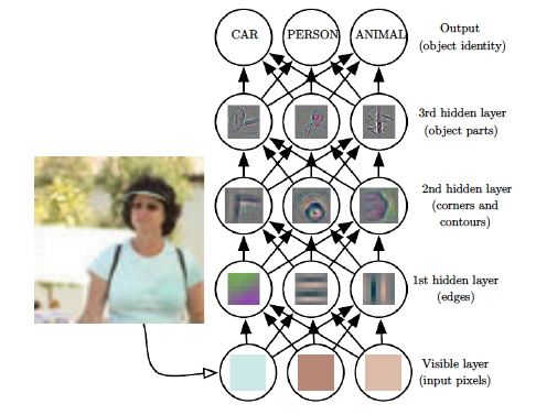
Figure 1.5: Hierarchical Processing of Images

The process that we described above by which DLN systems create higher level representations, works not just for images but also for language, i.e., DLNs can be used to create high level representations for words and sentences which capture semantic content. In particular it is possible to create DLN based representations for words by mapping them to vectors. Figure 1.6 graphs the 2-D representation of English words (once again using t-SNE to project onto 2 dimensions), after they have been processed by a DLN system. As in the case of images, the figure shows that the representation captures semantic information by clustering together words that are similar in meaning. This representation for words is widely used in Natural Language Processing (NLP) for doing tasks such as Machine Translation, Sentiment Analysis etc.

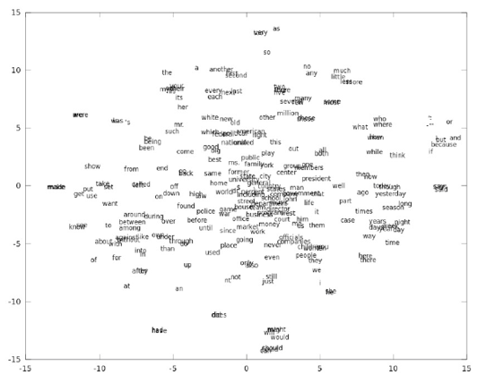
Figure 1.6: Word Representations

The rest of this monograph is organized as follows. In Chapter 2 we introduce DLN architecture by going through an example of the processing of MNIST images. In Chapter 3 we introduce the concepts of supervised and un-supervised learning, and set up the basic mathematical framework for training DLN models. In Chapter 4 we solve the simplest DLN models, i.e, those involving linear parameterization. Chapter 5 describes Fully Connected Neural Networks. Chapter 6 delves into the details of training DLNs, including a full description of the Backprop algorithm. Chapter 7 is on techniques that can be used to improve the Gradient Descent algorithm. In Chapter 8 we discuss the idea of Model Capacity, and its relation to the concepts of Model Underfitting and Model Overfitting. We discuss techniques used to optimally set the Learning Rate parameter, and other Hyper-Parameters in Chapter 9.

References

Sutskever, Ilya, Oriol Vinyals, and Quoc V. Le. 2014. “Sequence to Sequence Learning with Neural Networks.” NIPS, ArXiv:1409.3215 v3.

McCulloch, Warren, and Walter Pitts. 1943. “A Logical Calculus of the Ideas Immanent in Nervous Activity.” Bulletin Of Mathematical Biophysics 5: 115–33.

Rosenblatt, F. 1958. “The Perceptron: A Probabilistic Model for Information Storage and Organization in the Brain.” Psychological Review 65: 386–408.

Rosenblatt, F. 1962. Principles of Neurodynamics. New York, NY: Spartan.

Minsky, Marvin, and Seymour Papert. 1969. Perceptrons. Cambridge, MA: MIT Press.

Hahnloser, R., R. Sarpeshkar, M A Mahowald, R. J. Douglas, and H.S. Seung. 2000. “Digital Selection and Analogue Amplification Coesist in a Cortex-Inspired Silicon Circuit.” Nature, 947–51.

Nair, Vinod, and Geoffrey Hinton. 2010. “Rectified Linear Units Improve Restricted Boltzmann Machines.” ICML.

Srivastava, N. 2013. “Improving Neural Networks with Dropout.” Master’s Thesis, University of Toronto.