Chapter 3 Supervised Learning
Supervised Learning is one of the two major paradigms used to train Neural Networks, the other being Un-Supervised Learning. Supervised Learning is the easier problem to solve and historically appeared first with models such as the Perceptron. When progress in Supervised Learning stalled in the 80s and 90s due to the difficulties encountered in training DLNs with multiple Hidden Layers, researchers focused on Un-Supervised Learning and came up with systems such the Boltzmann Machine and its multiple Hidden Layer counterpart called Deep Belief Networks, see Roux and Bengio (2008); Roux and Bengio (2010). Indeed the breakthrough in 2006 that kicked off the current DLN renaissance occurred when it was shown that it is possible to train a DLN in a supervised fashion by using layer-by-layer un-supervised training, Hinton, Osindero, and Teh (2006). Since then advances in Supervised Learning have meant that it is now possible to train DLNs without resorting to Un-Supervised Learning. However it is widely recognized that in order to make further progress in DLNs, the next breakthroughs have to occur in the Un-Supervised Learning area, since it is difficult to get hold of the vast amounts of labeled data needed for Supervised Learning. In this chapter we set up the mathematical framework for the Supervised Learning problem, and then show how the problem can be solved using Statistical Estimation Theory and Optimization Theory.
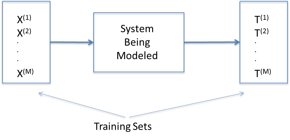
Figure 3.1: Supervised Learning
Consider the system shown in Figure 3.1. We assume that we don’t know anything about the internal working of the system, i.e., it exists as a black box. The only information we have about the system is that when it is subject to an input vector \(X{(m)}=(x_1{(m)},...,x_N{(m)}), 1 \leq m \leq M\) belonging to a Training Set, then it results in the vector \(T{(m)}=(t_1{(m)},...,t_K{(m)}), 1 \leq m \leq M\). The vector \(T{(m)}\) is called the “Ground Truth”, and corresponds to the “correct” output for the input \(X{(m)}\).
The vector \(T{(m)}\) is defined as follows: If the input vector \(X{(m)}\) belongs to the category \(q\), then \(t_q{(m)} = 1\) and \(t_k{(m)} = 0, k\neq q\). In the discussion below we sometimes also use the expression \(T{(m)} = q\) to refer the ground truth vector \(T{(m)}\) whose \(q^{th}\) component is \(1\) and the rest are \(0\). The Supervised Learning problem is defined as the process of synthesizing a model for the system based on these \(M\) input-output training pairs. This model should be such that if subject it to an input \(X\) (which is not one of the \(M\) training vectors), then it should result in a “correct” output \(T\).
The solution to the Supervised Learning problem proceeds in three steps:
The problem is recast using the framework of Statistical Estimation theory. This enables the formulation of the problem as an optimization problem.
A parametrized model is proposed for the system. The structure of the model is usually a creative breakthrough inspired by experimental results and/or intuitive insights. In the case of DLNs it has taken inspiration from what we understand about the workings of biological brains.
The parameters of the model in step (2) are estimated by solving the optimization problem from step (1).
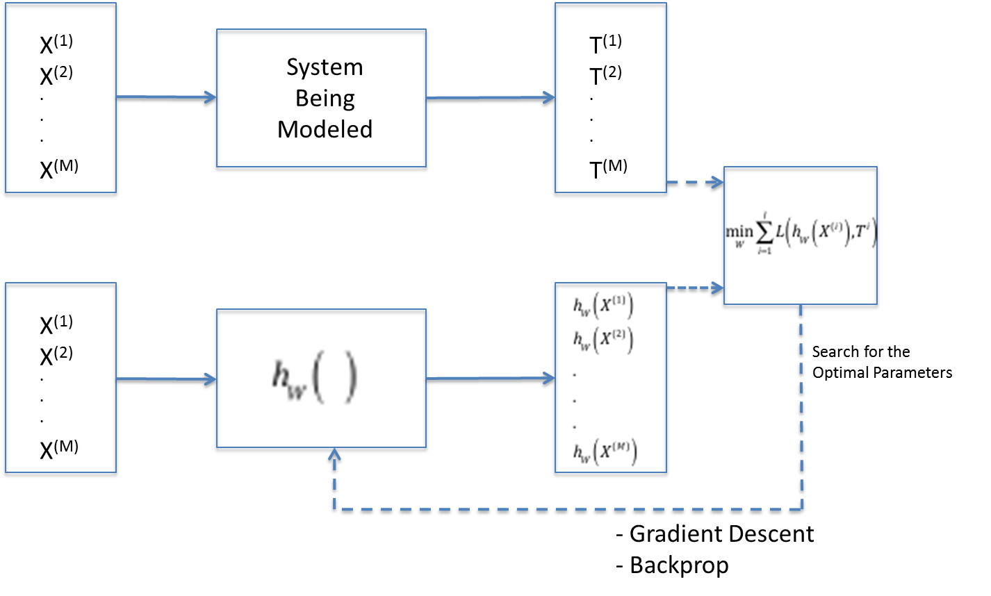
Figure 3.2: Solution to the Supervised Learning Problem
Figure 3.2 illustrates the formulation the Supervised Learning problem. The top half of the figure shows the system that is being modeled, the output \(T{(m)}\) of the system being the Ground Truth corresponding to the input \(X{(m)}\). The bottom half of the figure shows a DLN model \(h(X,W)\) for this system. Note that the subscript \(W\) represents the parameterization of the model. When we subject the model to the input \(X{(m)}\) , then it results in output vector \(h(X{(m)},W) = (h_1(X{(m)},W),...,h_K(X{(m)},W))\) for \(1 \leq i \leq M\).
3.1 Statistical Estimation Theory Formulation
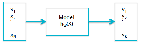
Figure 3.3: Probabilistic Formulation
In order to formulate the Supervised Learning problem in the framework of Statistical Estimation Theory, we start recasting the system model shown in the bottom half of Figure 3.2 within a probabilistic framework, as shown in Figure 3.3. The output vector \(Y = (y_1,...,y_K)\) of the model is defined by (ignoring the superscript \(m\) for the \(m^{th}\) sample for the moment) \[ y_k = P(T = k|X),\ \ 1\le k\le K \] \[ \sum_{k=1}^K y_k = 1 \] Hence we expect the model output \(Y\) to be a vector of conditional probabilities, such that the \(k^{th}\) component of \(Y\) is given by the conditional probability that the input vector \(X\) belongs to the category \(k\). We are asking the model to give us the conditional probabilities for the input \(X\) to belong to a particular class, as opposed to the actual system which outputs the Ground Truth with full certainity (see Figure 3.1). This formulation allows us to apply tools from Maximum Likelihood Estimation to the problem, which we do next.
Note that \[ P(T=(1,0,...,0)|X) = y_1 \] \[ P(T=(0,1,,...,0)|X) = y_2 \] . . . \[ P(T=(0,0,,...,1)|X) = y_K \] This set of equations can be written compactly as: \[ P(T=(t_1,...,t_K)|X) = (y_1)^{t_1} y_2^{t_2}\ ...\ y_K^{t_K} \] Using Maximum Likelihood Estimation Theory, the Likelihood function for this problem is given by product over all the samples in the training dataset. Re-introducing the superscript \(m\) for the \(m^{th}\) traning sample, we get the following expression for the Likelihood Function \(l\): \[ l = \prod_{m=1}^M P(T{(m)}|X{(m)}) = \prod_{m=1}^M \prod_{k=1}^K (y_k{(m)})^{t_k{(m)}} \] Taking the natural log on both sides, the Log Likelihood is given by \[ L = \log l = -{1\over M}\sum_{m=1}^M \sum_{k=1}^K t_k{(m)}\log y_k{(m)} \] Note the following: (1) Since \(0\le y_k{(m)}\le 1\), the negative sign ensures that the expression for \(L\) stays positive, and (2) We divide by \(M\) to average out the contribution from each training sample. Re-writing this equation using functional form for the model, we get \[ L(W) = -{1\over M}\sum_{m=1}^M \sum_{k=1}^K t_k{(m)}\log h_k(X{(m)},W) \] \(L(W)\) is referred to as the Loss Function (sometimes also called the Error Function) and it measures how close the model output \(Y\) are to the desired outputs \(T\). As per Maximum Likelihood Estimation Theory, the optimum parameters W are the ones that minimize \(L(W)\) (note that the negative sign changes the maximization to a minimization problem). Hence as shown in the box at the right hand side of Figure 3.2, \(L(W)\) is the expression that needs to be minimized in order to estimate the model parameters \(W\).
Note that the expression for the Loss Function \(L\) can be written as \[ L = {1\over M}\sum_{m=1}^M \mathcal{L}{(m)} \] where \[ \mathcal{L}{(m)} = -\sum_{k=1}^K t_k{(m)}\log y_k{(m)} \] The function \(\mathcal{L}\) is known as the Cross Entropy function, and is well known from the field of Information Theory, where it is used as a measure of the distance between probability distributions. The above expression says that the Loss Function \(L\) is obtained by averaging out the Cross Entropy between the distributions \(T{(m)}=(t_1{(m)},...,t_K{(m)})\) and \(Y{(m)}=(y_1{(m)},...,y_K{(m)})\) for a single sample of the dataset. Also note that if \(t_q{(m)} = 1\), then \(\mathcal L^{(m)}\) can be written as \[ \mathcal L{(m)} = -\log y_q{(m)} \] From this expression it is easy to see that if the two distributions match (i.e. the model’s prediction matches the ground truth), then \(\mathcal L{(m)} = 0\), while if there is mismatch, then the value of \(\mathcal L{(m)}\) increases steeply, and approaches infinity for a perfect mismatch (thus justifying its use as a measure of the mis-match).
At a high level, the process of mnimizing \(L\) and thereby finding the best set of parameters \(W\) (also called the Training Algorithm), is carried out in the following steps:
Given an input \(X(m)\), compute the model output \(Y(m)\).
Use \(Y(m)\) and the Ground Truth \(T(m)\) to compute the Cross Entropy \(\mathcal L\).
Tweak the parameters \(W\) so that \(\mathcal L\) value decreases
Repeat steps 1 to 3, until the Loss Function \(L\) drops below some threshold.
Given a family of models parametrized by W, we have reduced the problem of finding the best model to one of solving an optimization problem. A lot of the effort in Supervised Learning research has gone into finding efficient ways for solving this optimization problem, which can become non-trivial when the model contains millions of parameters. Since the 1980s, the most popular technique for solving this problem is the Backprop algorithm which is an efficient way to implement the classical Gradient Descent optimization algorithm in the DLN context. Backprop works by iteratively processing each training set pair \((X{(m)},T{(m)})\) and using this information to make incremental changes to the model parameter estimates in a fashion that causes the Loss Function to decrease.
As promised we have shown how to estimate the model parameters by using the training dataset. However this solves only half the problem, since we still haven’t revealed \(h(X,W)\) the functional form of the model. The rest of the monograph is devoted to addressing this. We start off with simple Linear Models in Chapter 4, and then move on to Deep Learning Models in Chapter 5. Convolutional Neural Networks are discussed in Chapter 12. These models work especially well for classifying images. Recurrent Neural Networks are discussed in Chapter 13. These models are well suited for detecting patterns in sequences of data, such those that arise in NLP applications.
References
Roux, N. Le, and Y. Bengio. 2008. “Representational Power of Restricted Boltzmann Machines and Deep Belief Networks.” Neural Computation 20 (6): 1631–49.
Roux, N. 2010. “Deep Belief Networks Are Compact Universal Approximators.” Neural Computation 22 (8): 2192–2207.
Hinton, G.E., S. Osindero, and Y. Teh. 2006. “A Fast Learning Algorithm for Deep Belief Nets.” Neural Computation 18: 1527–54.