Chapter 8 Training Neural Networks Part 2

Once the DLN model has been trained, its true test is how well it is able to classify inputs that it has not seen before, which is also known as its Generalization Ability. There are two kinds of problems that can afflict ML models in general:

1. Even after the model has been fully trained such that its training error is small, it exhibits a high test error rate. This is known as the problem of Overfitting.

2. The training error fails to come down in-spite of several epochs of training. This is known as the problem of Underfitting.

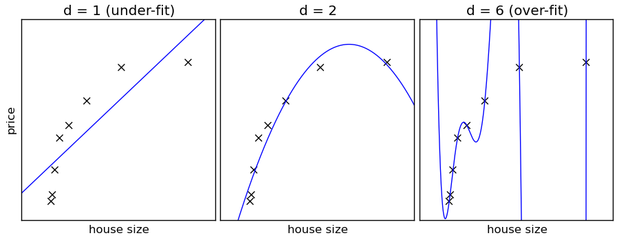
Figure 8.1: Illustration of Underfitting and Overfitting

The problems of Underfitting and Overfitting are best visualized in the context of the Regression problem of fitting a curve to the training data, see Figure 8.1. In this figure, the crosses denote the training data while the solid curve is the ML model that tries to fit this data. As shown, there are three types of models that were used to fit the data: A straight line in the left hand figure, a second degree polynomial in the middle figure and a polynomial of degree 6 in the right hand figure. The left figure shows that the straight line is not able to capture the curve in the training data, and leads to the problem of Underfitting, since even if we were to add more training data it won’t reduce the error. Increasing the complexity of the model by making the polynomial of second-degree helps a lot, as the middle figure shows. On the other hand if we increase the complexity of the model further by using a sixth-degree polynomial, then it backfires as illustrated in the right hand figure. In this case the curve fits all the training points exactly, but fails to fit test data points, which illustrates the problem of Overfitting.

This example shows that it is critical to choose a model whose complexity fits the training data, choosing a model that is either too simple or too complex results in poor performance. A full scale DLN model can have millions of parameters, and in this case a formal definition of its complexity reamins an open problem. A concept that is often used in this context is the that of “Model Capacity”, which is defined as the ability of the model to handle complex datasets. This can be formally computed for simple Binary Classification models and is known as the Vapnik-Chervonenkis or VC dimension. Such a formula does not exist for a DLN model in general, but later in this chapter we will give guidelines that can be used to estimate the effect of model’s hyper-parameters on its capacity.

The following factors determine how well a model is able to generalize from the training dataset to the test dataset:

• The model capacity and its relation to data complexity: In general if the model capacity is less than the data complexity then it leads to underfitting, while if the converse is true, then it can lead to overfitting. Hence we should try to choose a model whose capacity matches the complexity of the training and test datasets.

• Even if the model capacity and the data complexity are well matched, we can still encounter the overfitting problem. This is caused to due to an insufficient amount of training data.

Based on these observations, a useful rule of thumb is the following: The chances of encountering the overfitting problem increases as the model capacity grows, but decreases as more training data is available. Note that we are attempting to reduce the training error (to avoid the underfitting problem) and the test error (to avoid the overfitting problem) at the same time. This leads to conflicting demands on the model capacity, since training error reduces monotonically as the model capacity increases, but the test error starts to increase if the model capacity is too high. In general if we plot the test error as a function of model capacity, it exhibits a characteristic U shaped curve. The ideal model capacity is the point at which the test error starts to increase. This criteria is used extensively in DLNs to determine the best set of hyper-parameters to use.

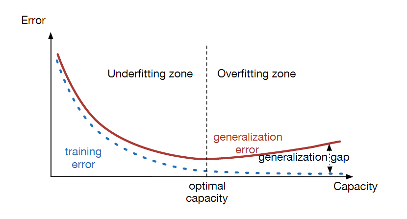
Figure 8.2: Model Capacity and its Effect on Underfitting and Overfitting

Figure 8.2 illustrates the tralationship between model capacity and the concepts of underfitting and overfitting by plotting the training and test errors as a function of model capacity. When the capacity is low, then both the training and test errors are high. As the capacity increases, the training error steadily decreases, but the test error initially decreases, but then starts to increases due to overfitting. Hence the optimal model capacity is the one at which the test error is at a minimum.

This discussion on the generalization ability of DLN models relies on a very important assumption, which is that both the training and test datasets can be generated the same probabilistic model. In practice what this means is that is we train the model to recognize a certain type of object, human faces for example, we cannot expect it to perform well if the test data consists entirely of cat faces. There is a famous result called the No Free Lunch Theorem that states that if this assumption is not satisfied, i.e., the training and test datasets distributions are un-constrained, then every classification algorithm has the same error rate when classifying previously unobserved points. Hence the only way to do better, is by constraining the training and test datasets to a narrower class of data that is relevant to the problem being solved.

8.1 The Validation Dataset

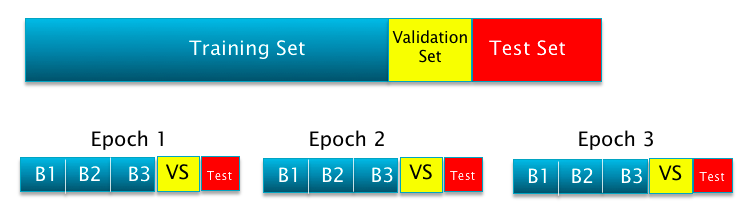
Figure 8.3: Illustrating the Validation Dataset

We introduced the validation dataset in Chapter 2, and also used it in Chapters 4 and 6 when describing the Gradient Descent algorithm. The reader may recall that the rule of thumb is to split the data between the training and test datasets in the ration 80:20, and then further set aside 20% of the resutling training data for the validation dataset (see Figure 8.3). We now provide some justification for why the validation dataset is needed.

During the course of this chapter we will often perform experiments whose objective is to determine optimal values of one or more hyper-parameters. We can track the variation of the error rate or classification accuracy in these experiments using the test dataset, but however this is not a good idea. The reason for this is that doing so causes information about the test data to leak into the training process. Hence we can ending up choosing hyper-parameters that are well suited for a particular choice of test data, but won’t work well for others. Using the validation dataset ensures that this leakage does not happen.

8.2 Detecting Underfitting

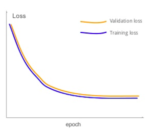
Figure 8.4: Model Underfitting

If a DLN exhibits the following symptom: Its training accuracy does not asymptote to zero, even when it is trained over a large number of epochs, then it is showing signs of underfitting. This means that the capacity of the model is not sufficiently high to be able to classify even the training data with a low probability of error. In other words, the degree of non-linearity in the training data is higher than the amount of non-linearity the DLN is capable of capturing. An example of the output from a model which suffers from underfitting is shown in Figure 8.4. As the figure shows both the training error and the validation error closely track each other, and flatten out to a large error value with increasing number of epochs. If the training and validation accuracies are plotted instead, they will also exhibit a synchronized flattening behavior while attaining only lower accuracy values.

In order to remedy this situation, the modeler can increase the model capacity by increasing the number of hidden layers, adding more nodes per hidden layer, changing regularization parameters (these are introduced in Section 8.4) or the Learning Rate. If these steps fail to solve the problem, then it points to bad quality training data.

8.3 Detecting Overfitting

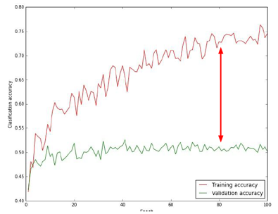
Figure 8.5: Detection of Overfitting

Overfitting is one of the major problems that plagues ML models. When this problem occurs, the model fits the training data very well, but fails to make good predictions in situations it hasn’t been exposed to before. The causes for overfitting were discussed in the introduction to this chapter, and can be boiled down to either a mismatch between the model capacity and the data complexity and/or insufficient training data. DLNs exhibit the following symptoms when overfitting happens (see Figure 8.5): The classification accuracy for the training data increases with the number of epochs and may approach 100%, but the test accuracy diverges and plateaus at a much lower value thus opening up a large gap between the two curves.

8.4 Regularization

In the previous section Regularization was introduced as a technique used to combat the Overfitting problem. We describe some popular Regularization algorithms in this section, which have proven to be very effective in practice. Because of the importance of this topic, there is a huge amount of work that has been done in this area. Dropout based Regularization which is described here, is one of the factors that has led to the resurgence of interest in DLNs in the last few years.

There are a wide variety of techniques that are used for Regularization, and in general the one characteristic that unites them is that these techniques reduce the effective capacity of a model, i.e., the ability for the model to handle more complex classification tasks. This makes sense since the basic cause of Overfitting is that the model capacity exceeds the requirements for the problem.

DLNs also exhibit a little understood feature called Self Regularization. For example for a given amount of Training Set data, if we increase the complexity of the model by adding additional Hidden Layers for example, then we should start to see overfitting, as per the arguments that we just presented. However, interestingly enough, increased model complexity leads to higher test data classification accuracy, i.e., the increased complexity somehow self-regularizes the model, see Bishop (1995). Hence when using DLN models, it is a good idea to start with a more complex model that the problem may warrant, and then add Regularization techniques if overfitting is detected.

Some commonly used Regularization techniques include:

• Early Stopping

• L1 Regularization

• L2 Regularization

• Dropout Regularization

• Training Data Augmentation

• Batch Normalization

The first three techniques are well known from Machine Learning days, and continue to be used for DLN models. The last three techniques on the other hand have been specially designed for DLNs, and were discovered in the last few years. They also tend to be more effective than the older ML techniques. Batch Normalization was already described in Chapter 7 as a way of Normalizing activations within a model, and it is also very effective as a Regularization technique.

These techniques are discussed in the next few sub-sections.

8.4.1 Early Stopping

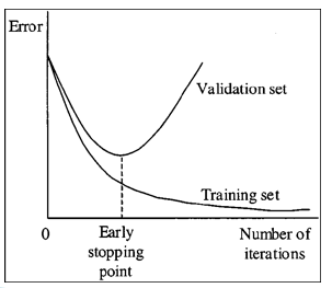
Figure 8.6: Early Stopping

Early Stopping is one of the most popular, and also effective, techniques to prevent overfitting. The basic idea is simple and is illustrated in Figure 8.6: Use the validation data set to compute the loss function at the end of each training epoch, and once the loss stops decreasing, stop the training and use the test data to compute the final classification accuracy. In practice it is more robust to wait until the validation loss has stopped decreasing for four or five successive epochs before stopping. The justification for this rule is quite simple: The point at which the validation loss starts to increase is when the model starts to overfit the training data, since from this point onwards its generalization ability starts to decrease. Early Stopping can be used by iteself or in combination with other Regularization techniques.

Note that the Optimal Stopping Point can be considered to be a hyper-parameter, hence effectively we are testing out multiple values of the hyper-parameter during the course of a single training run. This makes Early Stopping more efficient than other hyper-parameter optimization techniques which typically require a complete run of the model to test out a single hyper-parameyter value. Another advantage of Early Stopping is that it is a fairly un-obtrusive form of Regularization, since it does not require any changes to the model or objective function which can change the learning dynamics of the system.

8.4.2 L2 Regularization

L2 Regularization is a commonly used technique in ML systems is also sometimes referred to as “Weight Decay”. It works by adding a quadratic term to the Cross Entropy Loss Function \(\mathcal L\), called the Regularization Term, which results in a new Loss Function \(\mathcal L_R\) given by:

\[\begin{equation} \mathcal L_R = {\mathcal L} + \frac{\lambda}{2} \sum_{r=1}^{R+1} \sum_{j=1}^{P^{r-1}} \sum_{i=1}^{P^r} (w_{ij}^{(r)})^2 \tag{8.1} \end{equation}\]

The Regularization Term consists of the sum of the squares of all the link weights in the DLN, multiplied by a parameter \(\lambda\) called the Regularization Parameter. This is another Hyperparameter whose appropriate value needs to be chosen as part of the training process by using the validation data set. By choosing a value for this parameter, we decide on the relative importance of the Regularization Term vs the Loss Function term. Note that the Regularization Term does not include the biases, since in practice it has been found that their inclusion does not make much of a difference to the final result.

In order to gain an intuitive understanding of how L2 Regularization works against overfitting, note that the net effect of adding the Regularization Term is to bias the algorithm towards choosing smaller values for the link weight parameters. The value of the \(\lambda\) governs the relative importance of the Cross Entropy term vs the regularization term and as \(\lambda\) increases, the system tends to favor smaller and smaller weight values.

L2 Regularization also leads to more “diffuse” weight parameters, in other words, it encourages the network to use all its inputs a little rather than some of its inputs a lot. How does this help? A complete answer to this question will have to await some sort of theory of regularization, which does not exist at present. But in general, going back to the example of overfitting in the context of Linear Regression in Figure 8.1, it is observed that when overfitting occurs as in the right hand part of that figure, the parameters of the model (which in this case are coefficients to the powers of \(x\)) begin to assume very large values in an attempt to fit all of the training data. Hence one of the signs of overfitting is that the model parameters, whether they are DLN weights or polynomial coefficients, blow up in value during training, which results in the model giving too much importance to the idiosyncrasies of the training dataset. This line of argument leads to the conclusion that smaller values of the model parameters enable the model to generalize better, and hence do a better job of classifying patterns it has not seen before. This increase in the values of the model parameters always seems to occur in the later stages of the training process. Hence one of the effects of the Early Stopping rule is to restrain the growth in the model parameter values. Therefore, in some sense, Early Stopping is also a form of Regularization, and indeed it can be shown that L2 Regularization and Early Stopping are mathematically equivalent.

In order to get further insight into L2 Regularization, we investigate its effect on the Gradient Descent based update equations (6.3)-(6.4) for the weight and bias parameters. Taking the derivative on both sides of equation (8.1), we obtain

\[\begin{equation} \frac{\partial \mathcal L_R}{\partial w_{ij}^{(r)}} = \frac{\partial \mathcal L}{\partial w_{ij}^{(r)}} + {\lambda}\; w_{ij}^{(r)} \tag{8.2} \end{equation}\]

Substituting equation (8.2) back into (6.2), the weight update rule becomes:

\[\begin{equation} w_{ij}^{(r)} \leftarrow w_{ij}^{(r)} - \eta \; \frac{\partial \mathcal L}{\partial W_{ij}^{(r)}} - {\eta \lambda} \; w_{ij}^{(r)} \\ = \left(1 - {\eta \lambda} \right)w_{ij}^{(r)} - \eta \; \frac{\partial \mathcal L}{\partial w_{ij}^{(r)}} \tag{8.3} \end{equation}\]

Comparing the preceding equation (8.3) with equation (6.2), it follows that the net effect of the Regularization Term on the Gradient Descent rule is to rescale the weight \(w_{ij}^{(r)}\) by a factor of \((1-{\eta \lambda})\) before applying the gradient to it. This is called “weight decay” since it causes the weight to become smaller with each iteration.

If Stochastic Gradient Descent with batch size \(B\) is used then the weight update rule becomes

\[\begin{equation} w_{ij}^{(r)}\leftarrow \left(1 - {\eta \lambda} \right) w_{ij}^{(r)} - \frac{\eta}{B} \; \sum_{m=1}^B \frac{\partial \mathcal L(m)}{\partial w_{ij}^{(r)}} \tag{8.4} \end{equation}\]

In both preceding equations (8.3) and (8.4) the gradients \(\frac{\partial L}{\partial w_{ij}^{(r)}}\) are computed using the usual Backprop algorithm.

8.4.3 L1 Regularization

L1 Regularization uses a Regularization Function which is the sum of the absolute value of all the weights in DLN, resulting in the following loss function (\(\mathcal L\) is the usual Cross Entropy loss):

\[\begin{equation} \mathcal L_R = \mathcal L + {\lambda} \sum_{r=1}^{R+1} \sum_{j=1}^{P^{r-1}} \sum_{i=1}^{P^r} |w_{ij}^{(r)}| \tag{8.5} \end{equation}\]

At a high level L1 Regularization is similar to L2 Regularization since it leads to smaller weights. It results in the following weight update equation when using Stochastic Gradient Descent (where \(sgn\) is the sign function, such that \(sgn(w) = +1\) if \(w > 0\), \(sgn(w) = -1\) if \(w< 0\), and \(sgn(0) = 0\)):

\[\begin{equation} w_{ij}^{(r)} \leftarrow w_{ij}^{(r)} - {\eta \lambda}\; sgn(w_{ij}^{(r)}) - {\eta}\; \frac{\partial \mathcal L}{\partial w_{ij}^{(r)}} \tag{8.6} \end{equation}\]

Comparing equations (8.6) and (8.3) we can see that both L1 and L2 Regularizations lead to a reduction in the weights with each iteration. However the way the weights drop is different: In L2 Regularization the weight reduction is multiplicative and proportional to the value of the weight, so it is faster for large weights and de-accelerates as the weights get smaller. In L1 Regularization on the other hand, the weights are reduced by a fixed amount in every iteration, irrespective of the value of the weight. Hence for larger weights L2 Regularization is faster than L1, while for smaller weights the reverse is true. As a result L1 Regularization leads to DLNs in which the weight of most of the connections tends towards zero, with a few connections with larger weights left over. This type of DLN that results after the application of L1 Regularization is said to be “sparse”.

8.4.4 Dropout Regularization

Dropout is one of the most effective Regularization techniques to have emerged in the last few years, see Srivastava (2013); Srivastava et al. (2014). We first describe the algorithm and then discuss reasons for its effectiveness.

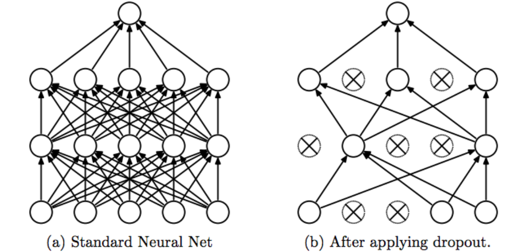
Figure 8.7: Dropout Regularization

The basic idea behind Dropout is to run each iteration of the Backprop algorithm on randomly modified versions of the original DLN. The random modifications are carried out to the topology of the DLN using the following rules:

• Assign probability values \(p^{(r)}, 0 \leq r \leq R\), which is defined as the probability that a node is present in the model, and use these to generate \(\{0,1\}\)-valued Bernoulli random variables \(e_j^{(r)}\): \[ e_j^{(r)} \sim Bernoulli(p^{(r)}), \quad 0 \leq r \leq R,\ \ 1 \leq j \leq P^r \]

• Modify the input vector as follows: \[\begin{equation} \hat x_j = e_j^{(0)} x_j, \quad 1 \leq j \leq N \tag{8.7} \end{equation}\]
• Modify the activations \(z_j^{(r)}\) of the hidden layer r as follows: \[\begin{equation} \hat z_j^{(r)} = e_j^{(r)} z_j^{(r)}, \quad 1 \leq r \leq R,\ \ 1 \leq j \leq P^r \tag{8.8} \end{equation}\]

The net effect of equation (8.7) is that for each iteration of the Backprop algorithm, instead of using the entire input vector \(x_j, 1 \leq j \leq N\), a randomly selected subset \(\hat x_j\) is used instead. Similarly the net effect of equation (8.8) is that, in each iteration of Backprop, a randomly selected subset of the nodes in each of the hidden layers is erased. Note that since the random subset chosen for erasure in each layer changes from iteration to iteration, we are effectively running Backprop on a different and thinned version of the original DLN network each time. This is illustrated in Figure 8.7, with Figure 8.7(a) showing the original DLN, and Figure 8.7(b) showing the DLN after a random subset of the nodes have been erased after applying Dropout. Also note that the erasure probabilities are the same for each layer, but can vary from layer to layer.

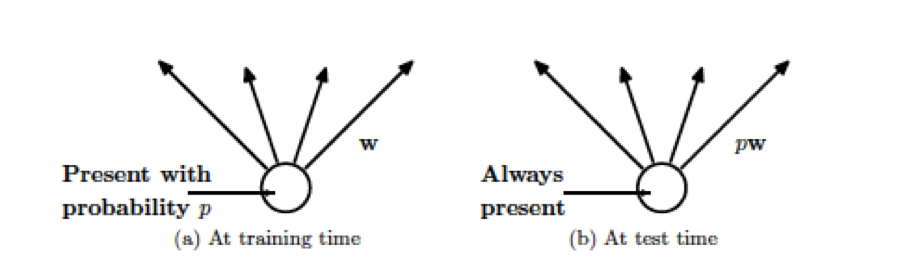
Figure 8.8: Weight Adjustment at Test time

After the Backprop is complete, we have effectively trained a collection of up to \(2^s\) thinned DLNs all of which share the same weights, where \(s\) is the total number of hidden nodes in the DLN. In order to test the network, strictly speaking we should be averaging the results from all these thinned models, however a simple approximate averaging method works quite well. The main idea is to use the complete DLN as the test network, but modify each of the weights as shown in Figure 8.8. Hence if a node is retained with probability \(p\) during training, then the outgoing weights from that link are multiplied by \(p\) at test time. This modification is needed since during the training period only a fraction \(p\) of the nodes are active at any one time, hence the average activation is only \(p\) times the value for the case when all the nodes are active, which is the case during the test phase. Hence by multiplting the test phase weights by \(p\), we insure that the average activation values are the same as during the training phase. Note that Dropout can be combined with other forms of Regularization such as L2 or L1, as well as other techniques that improve the Stochastic Gradient algorithm such as the learning rate momentum algorithm.

The complete Batch Stochastic Gradient Descent algorithm for Deep Feed Forward Networks using Dropout is given below:

1. Initialize all the weight and bias parameters \((w_{ij}^{(r)},b_i^{(r)})\).

2. For \(q = 0,...,{M\over B}-1\) repeat the following steps (2a) - (2f):

1. For the training inputs \(X_i(m), qB\le m\le (q+1)B\), compute the model predictions \(y(m)\) given by

\[ a_i^{(r)}(m) = \sum_{j=1}^{P^{r-1}} w_{ij}^{(r)}z_j^{(r-1)}(m)+b_i^{(r)}, \quad 2 \leq r \leq R,\ \ 1 \leq i \leq P^r \] and

\[ z_i^{(r)}(m) = e_i^{(r)}(m)f(a_i^{(r)}(m)), \quad 2 \leq r \leq R,\ \ 1 \leq i \leq P^r \]

and for \(r=1\),

\[ a_i^{(1)}(m) = \sum_{j=1}^{P^1} w_{ij}^{(1)}e_j^{(0)}(m)x_j(m)+b_i^{(1)} \quad \mbox{and} \quad z_i^{(1)}(m) = e_i^{(1)}(m)f(a_i^{(1)}(m)), \quad 1 \leq i \leq N \]

The logits and classification probabilities are computed as before using

\[ a_i^{(R+1)}(m) = \sum_{j=1}^K w_{ij}^{(R+1)}z_j^{(R)}(m)+b_i^{(R+1)}, \quad 1 \leq i \leq K \]

and

\[ \quad y_i(m) = \frac{\exp(a_i^{(R+1)}(m))}{\sum_{k=1}^K \exp(a_k^{(R+1)}(m))}, \quad 1 \leq i \leq K \]

Note that for each \(m\), a different set of erasure numbers \(e_i^{(r)}(m)\) are generated, so that the outputs \(Y(m),\ qB\le m\le (q+1)B\) are effectiveley generated using \(B\) different networks.

2. Evaluate the gradients \(\delta_k^{(R+1)}(m)\) for the logit layer nodes using

\[ \delta_k^{(R+1)}(m) = y_k(m) - t_k(m),\ \ 1\le k\le K \]

3. Back-propagate the \(\delta\)s using the following equation to obtain the \(\delta_j^{(r)}(m), 1 \leq r \leq R, 1 \leq j \leq P^r\) for each hidden node in the network.

\[ \delta_j^{(r)}(m) = e_j^{(r)}(m)f'(a_j^{(r)}(m)) \sum_k w_{kj}^{(r+1)} \delta_k^{(r+1)}(m), \quad 1 \leq r \leq R \] d. Compute the gradients of the Cross Entropy Function \(\mathcal L(m)\) for the \(m\)-th training vector \((X{(m)}, T{(m)})\) with respect to all the weight and bias parameters using the following equation.

\[ \frac{\partial\mathcal L(m)}{\partial w_{ij}^{(r+1)}} = \delta_i^{(r+1)}(m) z_j^{(r)}(m) \quad \mbox{and} \quad \frac{\partial \mathcal L(m)}{\partial b_i^{(r+1)}} = \delta_i^{(r+1)}(m), \quad 0 \leq r \leq R \]

5. Change the model weights according to the formula

\[ w_{ij}^{(r)} \leftarrow w_{ij}^{(r)} - \frac{\eta}{B}\sum_{m=qB}^{(q+1)B} \frac{\partial\mathcal L(m)}{\partial w_{ij}^{(r)}}, \] \[ b_i^{(r)} \leftarrow b_i^{(r)} - \frac{\eta}{B}\sum_{m=qB}^{(q+1)B} \frac{\partial{\mathcal L}(m)}{\partial b_i^{(r)}}, \]

Once again, due to the random erasures, we are averaging the gradients of \(B\) different networks in this step.

6. Increment \(q \leftarrow (q+1)\mod B\) and go back to step \((a)\).

3. Compute the Loss Function \(L\) over the Validation Dataset given by \[ L = -{1\over V}\sum_{m=1}^V\sum_{k=1}^K t_k{(m)} \log y_k{(m)} \]

where the outputs are computed using the formulae:

\[ a_i^{(r)}(m) = p^{(r-1)}\sum_{j=1}^{P^{r-1}} w_{ij}^{(r)}z_j^{(r-1)}(m)+b_i^{(r)}, \quad 2 \leq r \leq R,\ \ 1 \leq i \leq P^r \] and

\[ z_i^{(r)}(m) = f(a_i^{(r)}(m)), \quad 2 \leq r \leq R,\ \ 1 \leq i \leq P^r \] and for \(r=1\),

\[ a_i^{(1)}(m) = p^{(0)}\sum_{j=1}^{P^1} w_{ij}^{(1)}(m)x_j(m)+b_i^{(1)} \quad \mbox{and} \quad z_i^{(1)}(m) = f(a_i^{(1)}(m)), \quad 1 \leq i \leq N \] The logits and classification probabilities are computed using

\[ a_i^{(R+1)}(m) = p^{(R)}\sum_{j=1}^K w_{ij}^{(R+1)}z_j^{(R)}(m)+b_i^{(R+1)}, \quad 1 \leq i \leq K \]

and

\[ \quad y_i(m) = \frac{\exp(a_i^{(R+1)}(m))}{\sum_{k=1}^K \exp(a_k^{(R+1)}(m))}, \quad 1 \leq i \leq K \]

If \(L\) has dropped below some threshold, then stop. Otherwise go back to Step 2.

In most applications of Dropout, the number of parameters to be chosen is reduced to one, by making the following choices:

\[ p^{(0)} = 1, \ \ p^{(r)} = p,\ \ r = 1, 2,...,R \]

Under these assumptions only a single parameter \(p\) need be chosen, and it is usually defaulted to \(p = 0.5\).

Why does Dropout work? Once again we lack a complete theory of Regularization in DLNs that can be used to answer this question, but some plausible reasons are as follows:

• A popular technique that is often used in ML models is called “bagging”. In this technique several models for the problem under consideration are developed, each of them with their own parameters and trained on a separate slice of data. The test is then run on each model as well, and then the average of the outputs is used as the final result. The reader may notice that the Dropout algorithm accomplishes the same effect as training several different models, each with a different subset of the hidden nodes active, which may explain its effectiveness. Note that Dropout is only approximate bagging, since unlike in full bagging, all the models share their parameters and also some of their inputs.

• Another explanation for Dropout’s effectiveness is the following: During Dropout training, a hidden node cannot rely on the presence of other hidden nodes in order to be able to accomplish its task. Hence each hidden node must perform well irrespective of the presence of other hidden nodes, which makes them very robust and work in a variety of different networks, without getting too adapted to any one of them. This property helps in generalizing the classification accuracy from training to test data sets.

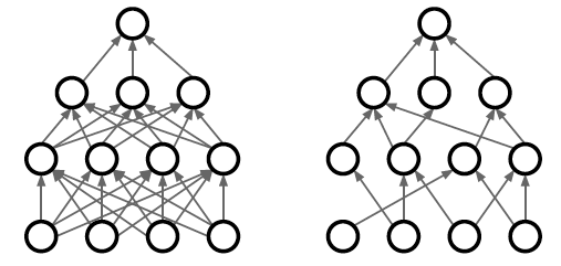
Figure 8.9: DropConnect Regularization

Since the invention of Dropout, researchers have introduced other Regularization techniques that work along similar lines. One such technique, called DropConnect, is shown in Figure 8.9. In this case, instead of randomly dropping nodes during training, random connections are dropped instead.

8.4.5 Training Data Augmentation

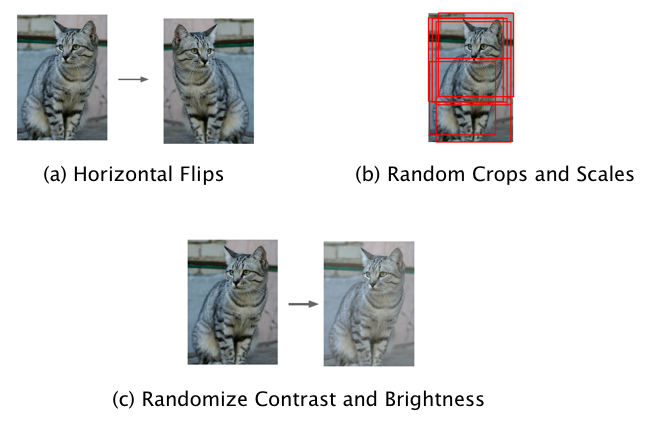
Figure 8.10: Data Augmentation for Images

If the data set used for training is not large enough, which is often the case for many real life test sets, then it can lead to overfitting. A simple technique to get around this problem is by artificially expanding the training set. In the case of image data, this fairly straightforward – for example we should be able to subject an image to the following transformation without changing its classification (see Figure 8.10 for some examples):

• Translation: Moving the image by a few pixels in various directions
• Rotation
• Reflection
• Skewing
• Scaling: Changing the size of the image while preserving its shape
• Changing contrast or brightness

All these transformations are of the type that the human eye is used to experiencing. However there are other augmentation techniques that don’t fall into this class, such as adding random noise to the training data set which is also very effective as long as it is done carefully.

All these techniques work quite well in practice. Later in Chapter 12 we will describe a DLN architecture called Convolutional Neural Networks (CNN) in which Translational Invariance is built into the structure of the network itself.

8.4.6 Model Averaging

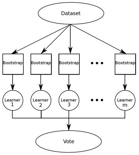
Figure 8.11: Bagging

Model Averaging is a well known technique from Machine Learning that is used to boost model accuracy. It relies on a result from statistics which states the following: Given random variables \(X_1,...,X_n\) with common mean \(\mu\) and variance \(\sigma\), the variance of the average \(\frac{\sum X_i}{n}\) of these variables is given by \(\sigma\over n\), i.e., the average becomess more deterministic as the number of random variables increases. Figure 8.11 shows how this result can be applied to ML models: If we train \(m\) models using \(m\) separate input datasets, and then use a simple majority vote to decide on the output, then it can lead to 2-5% improvement in model accuracy. This method can be further simplified in the following ways:

• Dividing up the input dataset reduces the number of samples per model which is not desirable. An alternative technique is to create input datasets for each model, by doing sampling with replacement. This results in each model having the same number of inputs as the original dataset, even though they may have samples that occur multiple time or samples that are absent in some of the datasets. This technique is commonly called “bagging”.

• An even simpler technique is to use the original input dataset in each of the models. This also works fairly well, since the randomness introduced due to factors such as the random initialization and the stochastic gradient algorithm, is sufficient to de-correlate the models.

8.4.7 Summary of Regularization

We end this section by making the observation that several Regularization techniques work by means of a two step procedure:

• Step 1: Introduce noise into the training procedure, which makes the system work harder in order to learn from the training samples. Examples include:

  • Dropout: Randomly drop nodes during training.

  • Batch Normalization: The data from a training sample is affected by the neighboring samples as a result of the normalization procedure.

  • Drop Connect: Randomly drop connections during training.

  • Model Averaging: Generate multiple models from the same training data, each of which has a different set of parameters, due to the use of random initializations and stochastic gradient descent.

• Step 2: At Test time, average out the randomness to generate final classification decision. Examples include:

  • Dropout: The final model used for testing is an approximation to the average of the randomly generated training models.

  • Batch Normalization: The final model is normalized using the entire test dataset, as opposed to normaliztion over batches during training.

  • Drop Connect: The final model is an approximation to the average of the randomly generated training models.

  • Model Averaging: Use a voting mechanism at test time to decide on the best classification.

References

Bishop, C.M. 1995. “Regularization and Complexity Control in Feed-Forward Networks.” Proceedings International Conference on Artificial Neural Networks ICANN’95 1: 141–48.

Srivastava, N. 2013. “Improving Neural Networks with Dropout.” Master’s Thesis, University of Toronto.

Srivastava, Nitish, Geoffrey Hinton, Alex Krizhevsky, Ilya Sutskever, and Ruslan Salakhutdinov. 2014. “Dropout: A Simple Way to Prevent Neural Networks from Overfitting.” J. Mach. Learn. Res. 15 (1). JMLR.org: 1929–58. http://dl.acm.org/citation.cfm?id=2627435.2670313.