Chapter 6 The Backprop Algorithm
In Chapter 4 we formulated the parameter estimation (or learning) problem for Linear Systems and showed that it could be solved using an optimization procedure based on the Gradient Descent algorithm. We now extend this framework to Deep Feed Forward Networks. Indeed all the arguments in Chapter 4 for Linear Systems continue to hold for Deep Feed Forward Networks, the only difference being that we can no longer use the simple gradient calculation \[ \frac{\partial \mathcal L}{\partial w_{ki}} = x_i(y_k - t_k) \] The gradients are instead computed by an algorithm called Backprop, which is probably the single most important algorithm in all of Deep Learning. Backprop was discovered in the mid-1980s, and since then the base algorithm hasn’t changed and it is still the most efficient technique that we know of to compute gradients in DLN systems.
In order to give an idea of the magnitude of the problem, consider a multi-layer Deep Learning model of the type discussed in Chapter 5. Models of this type can have millions of parameters: For example consider the case when the input is a 224x224x3 color image, and the model has a single Hidden Layer with 100 nodes. The number of weights in just the first layer of connections between the Input and the Hidden Layers is given by 224x224x3x100 = 15,082,800! In order to estimate these parameters from the training dataset, the gradients \(\frac{\partial\mathcal L}{\partial w_{ij}}\) with respect each one of these weights need to be calculated. This is a fairly daunting task, and a lack of solution stymied progress in DLN system until the mid-1980s. The logjam was finally broken with the discovery of the Backprop algorithm, see for example Montavon, Orr, and Müller (2012). Our objective is to derive this algorithm as well provide some intuition into the subject of Gradient Flows in general.
We start by stating the optimization problem for Deep Feed Forward Networks. The system parameters are estimated by solving the following optimization problem: Find the model parameters that minimize the Loss Function \(L\) given by: \[\begin{equation} L = {1\over M} \sum_{m=1}^M{\mathcal L}(m) \tag{6.1} \end{equation}\]where the Cross Entropy Function \(\mathcal L\) for the \(m^{th}\) training sample is given by \[ \mathcal L(m) = -\sum_{k=1}^K t_k(m)\log y_k(m) \] In this equation \((t_1(m),...,t_K(m))\) is the Label or Ground Truth vector and \((y_1(m),...,y_K(m))\) is the vector of classification probabilities, given by \[ y_k(m) = \frac{\exp(a_k(m))}{\sum_{j=1}^K\exp(a_j(m))},\ \ 1\le k\le K \] The numbers \((a_1(m),...,a_K(m))\) are the logits and are computed using a scoring function \(h_k\), so that \[ a_k(m) = h_k(W, b),\ \ 1\le k\le K \] The numbers \((W,b)\) represent the parameters that are used to specify the model. For Linear Systems the scoring functions were fairly simple: \[ a_k = \sum_{i=1}^N w_{ki}x_i + b_k,\ \ 1\le k\le K \]
For Deep Feed Forward Networks, these functions are much more complex. For example for a network with a single Hidden Layer the equations are \[ a_k = \sum_{i=1}^P w_{ki}^{(2)}z_i + b_k^{(2)},\ \ 1\le k\le K\,\ \ \mbox{where}\ \ z_i = f(\sum_{j=1}^N w_{ij}^{(1)}x_j + b_{i}^{(1)}),\ \ 1\le i\le P \]
where \(f\) is the Activation Function. This optimization problem is solved by using the Gradient Descent Algorithm, according to which the optimal parameters \((W,b)\) are estimated iteratively using the following equations:
\[\begin{equation} w_{ij}^{(r)} \leftarrow w_{ij}^{(r)} - \frac{\eta}{M}\sum_{m=1}^M \frac{\partial\mathcal L(m)}{\partial w_{ij}^{(r)}} \tag{6.2} \end{equation}\] \[ b_i^{(r)} \leftarrow b_i^{(r)} - \frac{\eta}{M}\sum_{m=1}^M \frac{\partial{\mathcal L}(m)}{\partial b_i^{(r)}} \] As was discussed in Chapter 4, there are two other Optimization Algorithms that are used in practice, since they converge faster than Gradient Descent, namely Stochastic Gradient Descent (SGD), given by \[\begin{equation} w_{ij}^{(r)} \leftarrow w_{ij}^{(r)} - \eta \frac{\partial{\mathcal L}(m)}{\partial w_{ij}^{(r)}} \tag{6.3} \end{equation}\] \[\begin{equation} b_i^{(r)} \leftarrow b_i^{(r)} - \eta \frac{\partial{\mathcal L}(m)}{\partial b_i^{(r)}} \tag{6.4} \end{equation}\] and Batch Stochastic Gradient Descent (B-SGD) with batch size \(B\), given by: \[\begin{equation} w_{ij}^{(r)} \leftarrow w_{ij}^{(r)} - \frac{\eta}{B}\sum_{m=qB}^{(q+1)B} \frac{\partial\mathcal L(m)}{\partial w_{ij}^{(r)}},\ \ 0\le q\le {M\over B}-1 \tag{6.5} \end{equation}\]\[ b_i^{(r)} \leftarrow b_i^{(r)} - \frac{\eta}{B}\sum_{m=qB}^{(q+1)B} \frac{\partial{\mathcal L}(m)}{\partial b_i^{(r)}}, \ \ 0\le q\le {M\over B}-1 \]
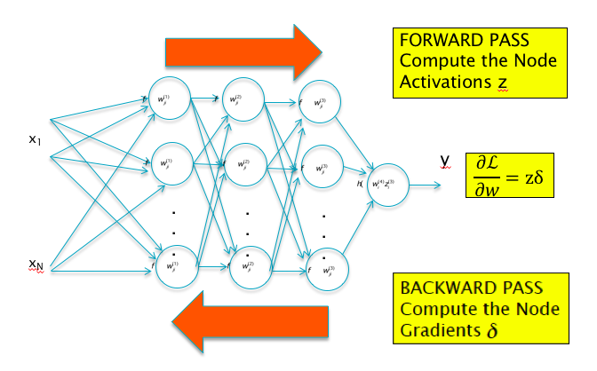
Figure 6.1: Backprop requires only two passes through the network irrespective of the number of parameters
In the absence of an explicit formula for \(\frac{\partial{\mathcal L}}{\partial w_{ij}^{(r)}}\), how do we proceed forward? A brute force approach to estimating these gradients is the following: Do a couple of forward passes through the network to compute \(\mathcal L(w_{11},...,w_{ij},..,w_{MN})\) and \(\mathcal L(w_{11},...,w_{ij} + \epsilon,..,w_{MN})\), where \(\epsilon\) is a small increment. Using these numbers the gradient with respect to \(w_{ij}\) can be estimated
\[ \frac{\partial {\mathcal L}}{\partial w_{ij}} = \frac{ {\mathcal L}(w_{11},...,w_{ij} + \epsilon,..,w_{MN}) - {\mathcal L}(w_{11},...,w_{ij},..,w_{MN})}{\epsilon} \] The reader can see that there is a problem with this scheme: If the network has a million parameters, then this requires a million and one forward passes through the network! The Backprop algorithm on the other hand, only requires just two passes through the network, irrespective of the number of parameters! As Figure 6.1 shows, Backprop requires a forward pass during which all the activations in the network are computed, and this is followed by a backward pass to the compute the gradients.
6.1 Gradient Flow Calculus
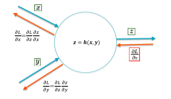
Figure 6.2: Gradient Flow Rules
Gradient Flow Calculus is the set of rules used by the Backprop algorithm to compute gradients (this also accounts for the use of the term “flow” in tools such as Tensor Flow). Backprop works by first computing the gradients \(\frac{\partial{\mathcal L}}{\partial y_{k}}, i\le k\le K\) at the output of the network (which can be computed using an explicit formula), then propagating or flowing these gradients back into the network. In this section we derive the rules that govern this backward flow of gradients.
Figure 6.2 shows a node with inputs \((x,y)\) and output \(z = h(x,y)\), where \(h\) represents the function performed at the node. Lets assume that the gradient \(\frac{\partial{\mathcal L}}{\partial z}\) is known. Using the Chain Rule of Differentiation, the gradients \(\frac{\partial{\mathcal L}}{\partial x}\) and \(\frac{\partial{\mathcal L}}{\partial y}\) can be computed as: \[ \frac{\partial{\mathcal L}}{\partial x} = \frac{\partial{\mathcal L}}{\partial z}\frac{\partial{z}}{\partial x} \] \[ \frac{\partial{\mathcal L}}{\partial y} = \frac{\partial{\mathcal L}}{\partial z}\frac{\partial{z}}{\partial y} \] This rule can be used to compute the effect of the node on the gradients flowing back from right to left. We apply these equtions to the following cases:
Addition \[z = x+y \] In this case \[ \frac{\partial{\mathcal L}}{\partial x} = \frac{\partial{\mathcal L}}{\partial y} = \frac{\partial{\mathcal L}}{\partial z} \] Hence the addition operation passes on the incoming gradient \(\frac{\partial{\mathcal L}}{\partial z}\) to all its input branches, without any modification. This is a simple result, but quite important in DLN architecture.
Multiplication by a Constant \[z = kx \] which results in \[ \frac{\partial{\mathcal L}}{\partial x} = k\frac{\partial{\mathcal L}}{\partial z} \] i.e, the multiplication operation in the forward direction results in an identical multiplication on the gradients flowing back.
Multiplication \[ z = xy \] In this case \[ \frac{\partial{\mathcal L}}{\partial x} = y\frac{\partial{\mathcal L}}{\partial z}, \ \ \mbox{and}\ \ \frac{\partial{\mathcal L}}{\partial y} = x\frac{\partial{\mathcal L}}{\partial z} \] Hence the multiplication operation also passes on the incoming gradient, but after multiplying it with the value from the other input branch.
The Max Operation \[ z = \max(x, y) \] \[ \frac{\partial{\mathcal L}}{\partial x} = \frac{\partial{\mathcal L}}{\partial z}\ \ if\ \ x > y\ \ \mbox{and}\ \ 0\ \ \mbox{otherwise} \] This shows that the max operation acts like a switch, so that the incoming gradient is switched to the input branch that is larger, while the other branch gets a zero gradient.
The Sigmoid Function \[ z = \sigma(x) = \frac{1}{1+\exp(-x)} \] In this case \[ \frac{\partial{\mathcal L}}{\partial x} = z(1-z)\frac{\partial{\mathcal L}}{\partial z} \] This equation has some very interesting implications for gradient flows for the case when the sigmoid is used as the Activation Function in DLNs. It implies that if the input value \(x\) is very large or very small, then the corresponding gradient \(\frac{\partial{\mathcal L}}{\partial x}\) goes to zero. We will see in the next chapter that this behavior held back progress in DLNs for almost two decades, even after the discovery of the Backprop algorithm.
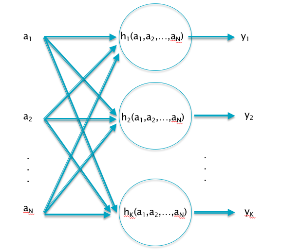
Figure 6.3: Multiple Inputs and Outputs
- Multiple Inputs and Multiple Outputs: Figure 6.3 shows a more complex case, in which there are \(K\) outputs, each of which are dependent on upto \(N\) inputs. In this case, the Chain Rule of Differentiation leads to the Gradient Flow Rule \[ \frac{\partial{\mathcal L}}{\partial a_i} = \sum_{k=1}^K \frac{\partial{\mathcal L}}{\partial y_k} \frac{\partial{y_k}}{\partial a_i} \] An important application of this Gradient Flow Rule is at the output of the Deep Feed Forward Network: \[ \mathcal L = -\sum_{j=1}^K t_j\log y_j,\ \ \mbox{and}\ \ y_j = \frac{\exp(a_j)}{\sum_{k=1}^K \exp(a_k)},\ \ 1\le j\le K \] Since these equations are also applicable to the output of Linear Models, the computation of \(\frac{\partial{\mathcal L}}{\partial a_i}\) was actually carried in Chapter 4 where we showed that \[ \frac{\partial{\mathcal L}}{\partial a_i} = y_i - t_i,\ \ 1\le i\le K \]
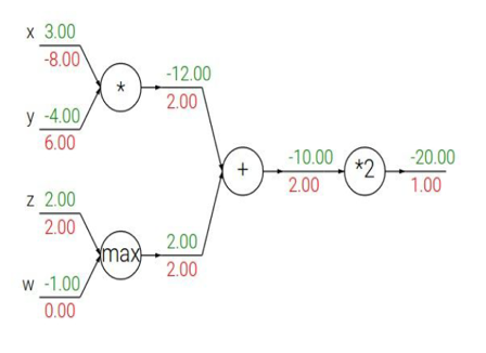
Figure 6.4: Gradient Flow Calculations
Figure 6.4 illustrates an application of the Gradient Flow rules to a simple neural network. The numbers in green represent the forward flow of activations, while the red numbers represent the backward flow of gradients.
6.2 Backprop
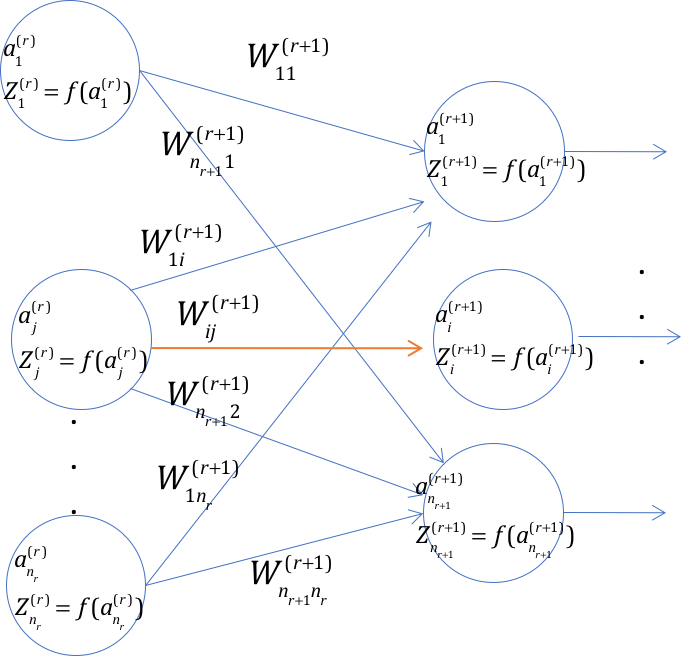
Figure 6.5: Step 1 in the derivation of Backprop equations
We are now ready to derive the equations for the Backprop algorithm, which we do in two steps.
Step 1
Consider Figure 6.5, where we show Hidden Layers \(r\) and \((r+1)\). Note that the highlighted link between the \(j\)-th node in layer \(r\), and the \(i\)-th node in layer \((r+1)\), has the weight \(w_{ij}^{(r+1)}\). Since the dependence of \(\mathcal L\) on this weight is only through the pre-activation \(a_i^{(r+1)}\), using the Chain rule of Differential Calculus, the derivative of the Cross Entropy Function \(\mathcal L\) with respect to this weight is given by:
\[\begin{equation} \frac{\partial\mathcal L}{\partial w_{ij}^{(r+1)}} = \frac{\partial\mathcal L}{\partial a_i^{(r+1)}} \cdot \frac{\partial a_i^{(r+1)}}{\partial w_{ij}^{(r+1)}} \tag{6.6} \end{equation}\] \[\begin{equation} \frac{\partial\mathcal L}{\partial b_i^{(r+1)}} = \frac{\partial\mathcal L}{\partial a_i^{(r+1)}} \cdot \frac{\partial a_i^{(r+1)}}{\partial b_i^{(r+1)}} \tag{6.7} \end{equation}\]Recall that \(a_i^{(r+1)} = \sum_j w_{ij}^{(r+1)} z_j^{(r)}+b_i^{(r+1)}\) where \(z_j^{(r)} = f(a_j^{(r)})\). It follows that
\[\begin{equation} \frac{\partial a_i^{(r+1)}}{\partial w_{ij}^{(r+1)}} = z_j^{(r)} \tag{6.8} \end{equation}\] \[\begin{equation} \frac{\partial a_i^{(r+1)}}{\partial b_i^{(r+1)}} = 1 \tag{6.9} \end{equation}\]Define the gradients \(\delta_i^{(r)}\) associated with node \(i\) in layer \(r\) by
\[\begin{equation} \delta_i^{(r)} = \frac{\partial\mathcal L}{\partial a_i^{(r)}} \tag{6.10} \end{equation}\]Then, from equations (6.6) - (6.10), it follows that
\[\begin{equation} \frac{\partial\mathcal L}{\partial w_{ij}^{(r+1)}} = \delta_i^{(r+1)} z_j^{(r)},\ \ r = 1,...,R \tag{6.11} \end{equation}\] \[\begin{equation} \frac{\partial\mathcal L}{\partial b_i^{(r+1)}} = \delta_i^{(r+1)},\ \ r = 1,...,R \tag{6.12} \end{equation}\]It can be easily shown that when \(r = 0\) (i.e., for the first Hidden Layer) the corresponding equation is
\[\begin{equation} \frac{\partial\mathcal L}{\partial w_{ij}^{(1)}} = \delta_i^{(1)} x_j \tag{6.13} \end{equation}\]because \(z_j^{(0)}=x_j\). From equations (6.11)-(6.12) it follows that the problem of computing the derivatives \(\frac{\partial\mathcal L}{\partial w}\) reduces to that of computing \(\delta_i^{(r)}\), \(1 \leq r \leq R\), \(1 \leq i \leq P^r\). This computation is done in Step 2.
Equations (6.11)-(6.13) are important results, they show that the gradient of the Loss Function with respect to the link weight \(w_{ij}^{(r+1)}\), is equal to the product of the following factors which are associated with the two ends of that link: The activation \(z_j^{(r)}\) associated with the left end of the link and the gradient \(\delta_i^{(r+1)}\) associated with the right end of the link (see Figure 6.6).
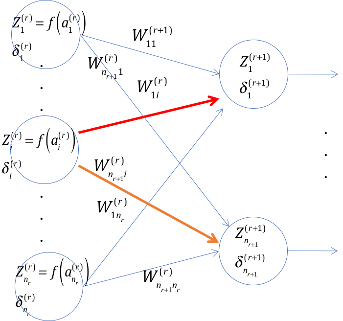
Figure 6.6: Step 2 in the derivation of Backprop equations
Step 2
In Step 2 we derive a recursive equation that can be used to compute the \(\delta\)s. Accordingly we assume that the gradients \(\delta_i^{(r+1)}, 1 \leq i \leq n_{r+1}\) at layer \((r+1)\) are known, and we back propagate these to compute \(\delta_i^{(r)}, 1 \leq i \leq n_r\) at layer \(r\). This computation falls within the Multiple Input Multiple Output framework of Gradient FLow Calculus (see previous section), however we will carry out the detailed calculations for completeness.
Since \(\mathcal L\) depends upon the sum \(a_i^{(r)}\) only through the corresponding sums \(a_j^{(r+1)}, 1 \leq j \leq n_{r+1}\) associated with nodes in layer \((r+1)\) (see Figure 6.6), using the chain rule of derivatives it follows that
\[\begin{equation} \delta_i^{(r)} = \frac{\partial\mathcal L}{\partial a_i^{(r)}} = \sum_{j=1}^{n_{r+1}} \frac{\partial\mathcal L}{\partial a_j^{(r+1)}} \cdot \frac{\partial a_j^{(r+1)}}{\partial a_i^{(r)}} \tag{6.14} \end{equation}\]Note that
\[\begin{equation} \frac{\partial\mathcal L}{\partial a_j^{(r+1)}} = \delta_j^{(r+1)} \tag{6.15} \end{equation}\]and since \(a_j^{(r+1)} = \sum_{i=1}^{P^r} w_{ji}^{(r+1)} z_i^{(r)} +b_j^{(r+1)}= \sum_{i=1}^{P^r} w_{ji}^{(r+1)} f(a_i^{(r)})+b_j^{(r+1)}\), it follows that
\[\begin{equation} \frac{\partial a_j^{(r+1)}}{\partial a_i^{(r)}} = f'(a_i^{(r)}) \cdot w_{ji}^{(r+1)} \tag{6.16} \end{equation}\]From equations (6.14)-(6.16) we obtain the following recursion:
\[\begin{equation} \delta_i^{(r)} = f'(a_i^{(r)}) \sum_{j=1}^{P^{r+1}} w_{ji}^{(r+1)} \delta_j^{(r+1)}, \quad 1 \leq r \leq R, 1 \leq i \leq P^r \tag{6.17} \end{equation}\]In order to initialize this recursion, the gradients \(\delta_k^{(R+1)}, 1 \leq k \leq K\) at the logit layer have to be computed. This calculation was done as part of the Multiple Inputs Multiple Outputs case in the previous section, and is as follows:
\[ \delta_k^{(R+1)} = \frac{\partial\mathcal L}{\partial a_k^{(R+1)}} = \sum_{j=1}^K\frac{\partial\mathcal L}{\partial y_j} \cdot \frac{\partial y_j}{\partial a_k^{(R+1)}} = y_k - t_k, \quad 1 \leq k \leq K \]
During the backward propagation part of the algorithm, we take this error between the actual output \(y_k\) and the ground truth \(t_k\), and then propagate it backwards, layer by layer.
6.3 Batch Stochastic Gradient Algorithm
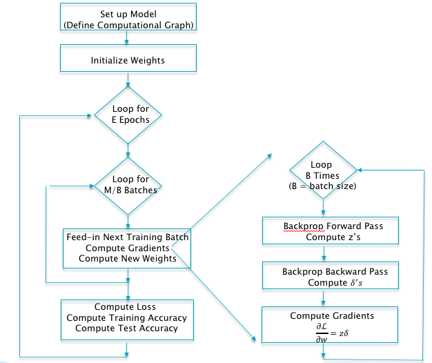
Figure 6.7: The Batch Stochastic Gradient Algorithm
The complete Batch Stochastic Gradient Descent algorithm for Deep Feed Forward Networks using Backprop is shown in Figure 6.7. The detailed steps are as follows:
Initialize all the weight and bias parameters \((w_{ij}^{(r)},b_i^{(r)})\) (this is a critical step, see Chapter 7 on how to do this).
For \(q = 0,...,{M\over B}-1\) repeat the following steps (2a) - (2f):
For the training inputs \(X_i(m), qB\le m\le (q+1)B\), compute the model predictions \(y(m)\) given by \[ a_i^{(r)}(m) = \sum_{j=1}^{P^{r-1}} w_{ij}^{(r)}z_j^{(r-1)}(m)+b_i^{(r)} \quad \mbox{and} \quad z_i^{(r)}(m) = f(a_i^{(r)}(m)), \quad 2 \leq r \leq R, 1 \leq i \leq P^r \] and for \(r=1\), \[ a_i^{(1)}(m) = \sum_{j=1}^{P^1} w_{ij}^{(1)}x_j(m)+b_i^{(1)} \quad \mbox{and} \quad z_i^{(1)}(m) = f(a_i^{(1)}(m)), \quad 1 \leq i \leq N \] The logits and classification probabilities are computed using \[ a_i^{(R+1)}(m) = \sum_{j=1}^K w_{ij}^{(R+1)}z_j^{(R)}(m)+b_i^{(R+1)} \quad \mbox{and} \quad y_i(m) = \frac{\exp(a_i^{(R+1)}(m))}{\sum_{k=1}^K \exp(a_k^{(R+1)}(m))}, \quad 1 \leq i \leq K \] This step constitutes the forward pass of the algorithm.
Evaluate the gradients \(\delta_k^{(R+1)}(m)\) for the logit layer nodes using \[ \delta_k^{(R+1)}(m) = y_k(m) - t_k(m),\ \ 1\le k\le K \] This step and the following one constitute the start of the backward pass of the algorithm, in which we compute the gradients \(\delta_k^{(r)}, 1 \leq k \leq K, 1\le r\le R\) for all the hidden nodes.
- Back-propagate the \(\delta\)s using the following equation to obtain the \(\delta_j^{(r)}(m), 1 \leq r \leq R, 1 \leq j \leq P^r\) for each hidden node in the network. \[ \delta_j^{(r)}(m) = f'(a_j^{(r)}(m)) \sum_k w_{kj}^{(r+1)} \delta_k^{(r+1)}(m), \quad 1 \leq r \leq R \]
- Compute the gradients of the Cross Entropy Function \(\mathcal L(m)\) for the \(m\)-th training vector \((X{(m)}, T{(m)})\) with respect to all the weight and bias parameters using the following equation. \[ \frac{\partial\mathcal L(m)}{\partial w_{ij}^{(r+1)}} = \delta_i^{(r+1)}(m) z_j^{(r)}(m) \quad \mbox{and} \quad \frac{\partial \mathcal L(m)}{\partial b_i^{(r+1)}} = \delta_i^{(r+1)}(m), \quad 0 \leq r \leq R \]
- Change the model weights according to the formula \[ w_{ij}^{(r)} \leftarrow w_{ij}^{(r)} - \frac{\eta}{B}\sum_{m=qB}^{(q+1)B} \frac{\partial\mathcal L(m)}{\partial w_{ij}^{(r)}}, \] \[ b_i^{(r)} \leftarrow b_i^{(r)} - \frac{\eta}{B}\sum_{m=qB}^{(q+1)B} \frac{\partial{\mathcal L}(m)}{\partial b_i^{(r)}}, \]
Increment \(q\leftarrow (q+1)\mod B\) and go back to step \((a)\).
- Compute the Loss Function \(L\) over the Validation Dataset given by \[ L = -{1\over V}\sum_{m=1}^V\sum_{k=1}^K t_k{(m)} \log y_k{(m)} \] If \(L\) has dropped below some threshold, then stop. Otherwise go back to Step 2.
The algorithm described above was known by the mid-1980s. Even then it took about two more decades before we had the Deep Learning Renaissance. The next two chapters go into reasons why this was the case. Specifically, there are a number of additional considerations involved in using the Backprop algorithm, including:
- Choosing a good Activation Function: This is a critical choice, we will examine various alternatives in Chapter 7.
- Regularization: In our description of Backprop we left out an important detail, i.e., the topic of Regularization. It determines how well the model is able to generalize its learning from the training data, to be able to accurately classify test data that it has not seen before. Since this is a fairly big topic in itself, we devote all of Chapter 8 to it.
- Choosing Hyper-Parameter values: So far we have come across the following hyper-parameters: The Learning Rate \(\eta\), the number of Hidden Layers \(R\) and the number of nodes per Hidden Layer \(P^r\), and in the following chapters we will add Regularization related parameters to this list. Part of the DLN training process is choosing good values for them.
- Initializing the weight parameters: All the weight and bias parameters have to be initialized at the start of the algorithm. If not done properly, it can cause the gradients to converge to zero, which terminates the training process.
- The stopping problem: This is the problem of when to stop the optimization process and conclude that further training won’t help improve the accuracy of the model.
Why does Gradient Descent work so well for DLNs? Gradient based optimization algorithms are guaranteed to find the minimum if the Loss Function is strictly convex with a global minimum. In reality, the Loss Function in DLNs is highly complex and possesses multiple minima, so that there is a danger that the optimization will get stuck in one of them. In practice this does not seem to matter since the algorithm nevertheless works very well, and it is not clear why this is the case. A theory that has been put forward to explain this is that the stochastic batch gradient descent technique, i.e., equations (6.3)-(6.4), introduces randomness into the algorithm, so that occasionally the algorithm may move in non-optimal directions. This increases the probability that if it enters a non-optimum local minima, then it may pop out of it. In all likelihood the algorithm does not settle into the global minima, however it does not seem to make much difference to its efficacy if it finds it way to a local minima. Another explanation that has been put forward to explain the unreasonable effectiveness of Gradient Descent is the following: For smaller models the Loss function exhibits minima that vary in size, so that finding the global minima is important. However models with millions of parameters have a fundamentally different distribution of Loss Function minima. Indeed as the model grows larger, all the minima seem to converge to similar values, so it does not matter which minima the algorithm ends up in.
References
Montavon, Grégoire, Genevieve B. Orr, and Klaus-Robert Müller, eds. 2012. Neural Networks: Tricks of the Trade - Second Edition. Vol. 7700. Lecture Notes in Computer Science. Springer. doi:10.1007/978-3-642-35289-8.