Chapter 5 Deep Feed Forward Networks
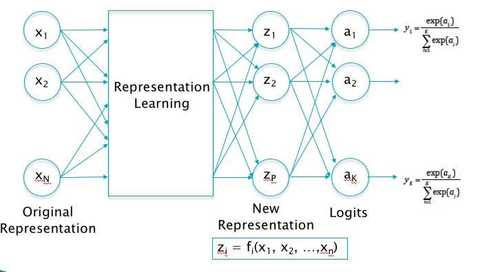
Figure 5.1: Transitioning to Deep Learning
The Linear Models that we discussed in Chapter 4 work well if the input dataset is approximately linearly separable, but they have limited accuracy for complex datasets. Some of the issues with Linear Models are the following:
If the input data is not linearly separable, then the designer has to expend a lot of effort in finding an appropriate feature map that makes it so. It would be nice to have a model that solves this problem automatically, by learning the best feature map from the data itself.
We showed that the model weight parameters could be regarded as a filter, so that for \(K\) classes, the operation of the system is equivalent to trying to the match the input with \(K\) different filters. The limitations of this approach can be seen in the filter for the “horse” class in Figure 4.8. The filter looks like a horse with two heads, since it is trying its best to match with a horse image, irrespective of the direction in which the horse is facing. This type of filtering will clearly not work for cases in which the horse were standing with some other orientation, or if it were located in a corner of the image. The fact that the best accuracy that can be achieved with linear classifiers and the CIFAR-10 Dataset is only about 40% is a reflection of this shortcoming. The linear system tries to do classification by taking each and every pixel into account, which is a difficult task. What if it were possible to create representations for higher level features in the image, say the head of the horse or its legs, and then use these for classification instead. This will enable the system to identify a horse irrespective of its orientation and its location in the image. This is precisely what Deep Learning systems do.
In general a way to make any model more powerful is by increasing the number of parameters. However in a Linear Model the number of parameters is constrained to \(KN + K\) by the sizes of the input data and the number of output classes, which limits its modeling power.
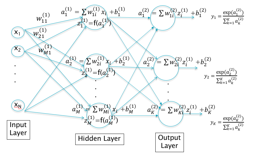
Figure 5.2: A Deep Feed Forward Network with One Hidden Layer
Deep Feed Forward Networks were designed with the objective the overcoming these shortcomings. As Figure 5.1 shows, we are looking for a functional block between the input vector \((x_1,...,x_N)\) and the output logits \((a_1,...,a_K)\), that can create a new representation vector \((z_1,...,z_P)\) which satisfies the approximate linear separability property. One way to do this is shown in Figure 5.2, which is a Deep Feed Forward Network with a single Hidden Layer. Note the following:
The Input layer and Output layers are as before, but we have added a third layer, the so-called Hidden Layer in between. The Input Layer is fully connected to the Hidden Layer, i.e., each node in the Input Layer is connected to every other node in the Hidden Layer, and the same holds true for connections between the Hidden Layer and the Output Layer. DLNs with these characteristics are called Deep Fully Connected Feed Forward Neural Networks. Later in this monograph we will come across examples of DLNs where these properties don’t apply; either because the fully connected property does not hold (as in Convolutional Neural Networks), or the DLN incorporates feedback loops (as in Recurrent Neural Networks).
The \(j\)-th node in the Hidden Layer performs the following computation on the input variables \(x_i\) to generate an output \(z_j^{(1)}, 1 \leq j \leq P\) given by \[ a_j^{(1)} = \sum_{i=1}^N w_{ji}^{(1)} x_i + b_j^{(1)} \] \[ z_j^{(1)} = f(a_j^{(1)}) \] The vector \((a^{(1)}_1,...,a_P^{(1)})\), which we call the Pre-Activation, is computed as a simple linear combination of the Input Vector. The output of the Hidden Layer \((z^{(1)}_1,...,z_P^{(1)})\) which we call the Activation, is computed as an elementwise non-linear function of the Pre-Activations.
The Output Layer operates on the Activations \(z_j^{(1)}\) from the Hidden Layer, and computes the logits for the K classes \((a_1^{(2)},...,a_K^{(2)})\). \[ a_k^{(2)} = \sum_{i=1}^P w_{ki}^{(2)} z_i^{(1)} + b_k^{(2)}, \ \ 1\le k\le K \] The classification probabilities \(y_k, 1\le k\le K\) are obtained by applying the Softmax function to the logits. \[ y_k = \frac{\exp(a_k^{(2)})}{\sum_{j=1}^K \exp(a_j^{(2)})}, \ \ 1\le k\le K \] Note that the logit and classification probability computations are identical to that done in Linear Systems, with the inputs \(X\) now replaced by the activations \(Z\).
The weight parameters \(w_{ij}^{(1)}, 1\le i\le P,1\le j\le N; w_{ij}^{(2)}, 1\le i\le K,1\le j\le P\) and the bias parameters \(b_i^{(1)}, 1\le i\le P; b_i^{(2)}, 1\le i\le K\) have to be learnt using the training data, as in Linear Models. The total number of parameters need to describe this network is given by \(NP + P + PK + K\), which is now dependent on the number of nodes in the Hidden Layer \(P\). Hence we can build a Deep Feed Forward model with more powerful classification ability by increasing the number of nodes in the Hidden Layer, which is an option that does not exist in Linear Systems.
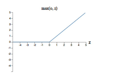
Figure 5.3: The ReLU Function
The activations \((z^{(1)}_1,...,z_P^{(1)})\) correspond to the new data representation that we are looking for. They filter the input and create higher layer representations, which are then used by the logit layer for classification. Note that the filtering done by the Hidden Layer is non-linear due to the presence of the non-linear Function \(f\). This function is called the Activation Function, and plays an important role in system performance. The most popular Activation Function in use is called the Rectified Linear Unit, or ReLU, and is shown in Figure 5.3. It simply passes on the pre-activations that are greater than zero, and blocks those that are less. The presence of the Activation Function is critical to the functioning of the DLN, and it can be easily shown that if they were to be omitted, then the Hidden and Output layers can be collapsed together so that the resulting model would be equivalent to a Linear Model. Indeed the presence of Activation Functions gives the system its modeling power, and in general we will see later in the book that DLN systems can be made more powerful by increasing the amount of non-linear processing. The appropriate choice of Activation Functions has a big influence on the performance of the DLN, and the discovery of more effective Activation Functions such as the ReLU have helped make DLNs easier to train.
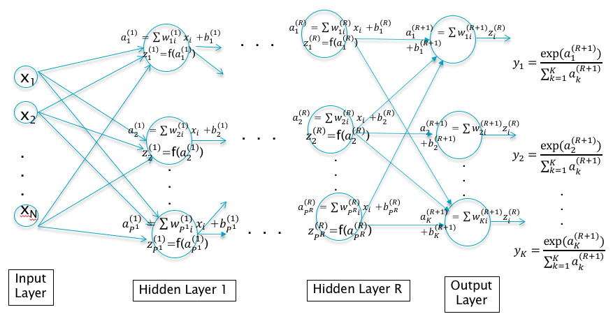
Figure 5.4: A Deep Feed Forward Network with R Hidden Layers
The system shown in Figure 5.2 incorporates only a single Hidden Layer. Why not continue the process and enable the model to create higher level representations by adding additional hidden layers. This is certainly possible and the resulting network is shown in Figure 5.4. It shows a Deep Feed Forward Network with \(R\) hidden layers, such that layer \(r\) consists of \(P^r\) nodes. The equations decribing this network can be written as:
- The activations for the first Hidden Layer: \[ a_j^{(1)} = \sum_{i=1}^N w_{ji}^{(1)} x_i + b_j^{(1)},\ \ 1\le j\le P^1 \] \[ z_j^{(1)} = f(a_j^{(1)}),\ \ 1\le j\le P^1 \]
- The Activations for Hidden Layer 2 to Hidden Layer R: \[ a_j^{(r+1)} = \sum_{i=1}^{P^r} w_{ji}^{(r+1)} z_i^{r} + b_j^{(r+1)},\ \ 1\le r\le R-1, 1\le j\le P^{(r+1)} \] \[ z_j^{(r+1)} = f(a_j^{(r+1)}),\ \ 1\le r\le R-1, 1\le j\le P^{(r+1)} \]
- The logits and the classification probabilities: \[ a_k^{(R+1)} = \sum_{i=1}^{P^R} w_{ki}^{(R+1)} z_i^R + b_k^{(R+1)},\ \ 1\le k\le K \] \[ y_k = \frac{a_k^{(R+1)}}{\sum_{j=1}^K a_j^{(R+1)}}, \ \ 1\le k\le K \]
With each successive Hidden Layer, this network creates representations at higher levels of abstraction.
We have introduced two degrees of freedom in DLN design in this chapter: (1) The number of Hidden Layers, and (2) The number of nodes per Hidden Layer. This leads to the following questions:
- To get a better performing model, is it preferable to increase the number of layers, or is it better to increase the number of nodes per layer (while keeping the number of layers fixed)?
- Does the system performance keep improving as we add more and more layers, or are there limits that the model runs into?
Unfortunately there don’t exist many theoretical results in this area which can give definite answers to these questions. However there is one interesting theorem regarding Deep Feed Forward Networks with a single Hidden Layer whose proof was given by Cybenko et.al. in 1989:
Given an arbitrary continuous function \(g\) of \(n\) variables such as \[ y = g(x_1,...,x_n) \]
it is always possible to find a Deep Feed Forward Network with a single Hidden Layer, such that the output of the network approximates \(g\), and the approximation can be made as close as we want by adding nodes to the Hidden Layer.
This property is of course dependent on the form of the Activation Function used, but it has been proven to be true for the most commonly used functions. Hence it should be possible to solve any classification problem with a Deep Feed Forward Network containing a single layer. However the theorem does not specify the number of hidden nodes needed for a particular problem.
In practice, the following has been observed that to increase the modeling power of a DLN, it is always better to add Hidden Layers, as opposed to increasing the number of nodes per Hidden Layer, becuase the former results in a network with a smaller number of parameters. We will see later in Chapter 8, that networks with more parameters require larger Training Datasets in order to avoid a problem called Overfitting, hence it is always preferable to have a model with a smaller number of parameters. Based on the previous discussion, there are many reasons why a DLN with more Hidden Layers is more powerful, among them:
More layers allow the model to develop an hierarchical representation of the input data, which simplifies the task of the linear classifier in the final layer.
Having additional layers increases the amount of non-linearity and thus the modeling capacity.
The other question that we raised is whether the DLN performance keeps improving as we add more and more Hidden Layers. This is actually not the case, the model performance is constrained due to the following factors:
The Vanishing Gradient Problem: In order to train a multilayer Deep Feed Forward Network, the gradients \(\frac{\partial L}{\partial w^{(r)}_{ij}}\) and \(\frac{\partial L}{\partial b^{(r)}_i}\) have to be computed. It turns that if the number of layers is large, the gradients of the weights that are either in the first few layers or the last few layers, converge towards zero as the trainig progresses. Once this happens, the corresponding weights stop adapting to new training data, and thus the training process grinds to a halt. This phenomena is known as the Vanishing Gradient problem, and its causes are explained in detail in Chapter 7. This problem contrains the number of layers that can be added to the network to asbout 20 or so, without degrading the training process. There has been a recent advance in DLN architecture called Residual Netwrks (or ResNets) which allows much deeper networks containing hundreds of layers.
The Overfitting Problem: Larger models with more layers have a larger number of parameters, and this in turn requires larger training datasets. As explained in Chapter 8, modeling is an exercise in matching the Capacity of the Model with the Complexity of the Dataset. If the Capacity of the Model is greater than the Complexity of the Dataset (which can happen if we add more layers than necessary), then it leads to overfitting. This problem constrains the model’s generalization ability.
As this discussion shows, there is no formula or theoretical result which tells us the number of layers or the nodes per layer to use in the model. These numbers, which are also called hyper-parameters are a function of the dataset that we are trying to model, and the only way to find the best numbers is by trial and error. Hence when building the model, the designer has to do several trial runs with different vales for these hyper-parameters before settling on the best ones. In Chapter 8 we provide some guidelines that can be used to make this process more efficient.