Chapter 9 Training Neural Networks Part 3

In the last few chapters we described some DLN models and algorithms that can be used to train them. We also expounded on ways to improve the training process by means of proper parameter initializations and techniques such as Regularization and Adam based optimization. However if a practitioner where to attempt to build a model, there are still a number of questions that have to be answered, such as:

1. What is the best model for the problem to be solved?

2. Given the plethora of training algorithms, such as Momentum, Adam, Batch Normalization, Dropout etc., which are the ones that are most appropriate for the model?

3. How much data is sufficient to train the model?

4. How should we select the various parameters associated with the model? These include:

   • Model topology related parameters such as the number of hidden layers and the number of nodes per hidden layer.
   • Training related parameters such the Learning Rate, Momentum parameter, Regularization parameters, Batch Size, Stopping Time etc.

   All these parameters are collectively known as hyper-parameters.

We attempt to answer these questions in this chapter and towards the end we provide some practical tips for de-bugging DLN models.

9.1 Choosing the Model

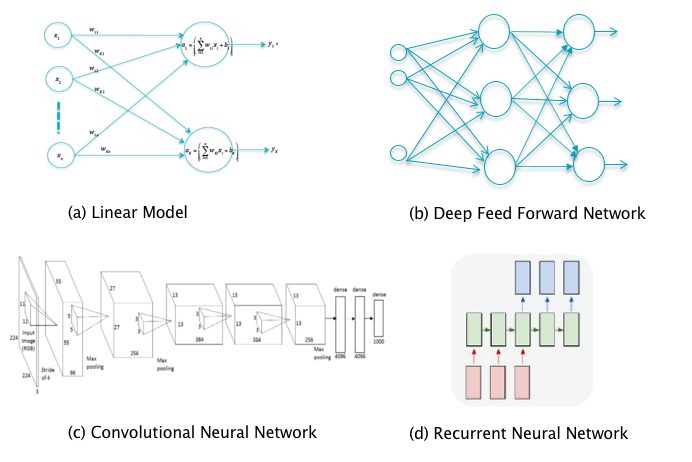
Figure 9.1: Choosing the Model

There are a number of options with regards to model choice (see Figure 9.1):

• If the input data is such that the various classes are approximately linearly separated (which can verified by plotting a subset of input data points in two dimensions using projection techniques), then a linear model will work.

• Deep Learning Networks are needed for more complex datasets with non-linear boundaries between classes. If the input data has a 1-D structure, then a Deep Feed Forward Network will suffice (see Chapter 5).

• If the input data has a 2-D structure (such as black and white images), or a 3-D structure (such color images), then a Convolutional Neural Network or ConvNet (see Chapter 12) is called for. In some cases 1-D or 2-D data can be aggregated into a higher level structure which then becomes amenable to processing using ConvNets. ConvNets excel at object detection and recognition in images and they have also been applied to tasks such as DLN based image generation.

• If the input data forms a sequence with dependencies between the elements of the sequence, then a Recurrent Neural Network or RNN is required (see Chapter 13). Typical examples of this kind of data include: Speech waveforms, natural language sentences, stock prices etc. RNNs are ideal for tasks such as speech recognition, machine translation, captioning etc

The basic structures described above can be combined in various ways to generate more complex models. For example if the input sequence consists of correlated 2-D or 3-D data structures (such as individual frames in a video segment), then the appropriate structure is a combination of RNNs with ConvNets. Another well know hybrid structure is called Network-in-a-Network and consists of a combination of ConvNets with Deep Feed Forward Networks. In recent years the number of models has exploded with new structures that advance the state of the art in various directions, such as enabling better gradient propagation during Backprop, and we will describe some of these in Chapters 12 and 13.

9.2 Choosing the Algorithms

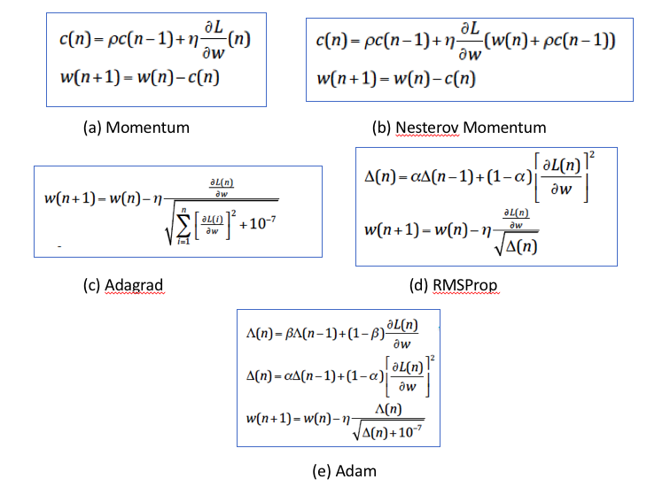
Figure 9.2: Choice of Stochastic Gradient Descent Parameter Update Equation

We have a choice of algorithm in the following areas:

• Choice of Stochastic Gradient Descent Parameter Update Equation: The parameter update equations discussed in Chapter 7 are shown in Figure 9.2. Of these Momentum and Nesterov Momentum are designed to speed up the speed of convergence and Adagrad and RMProp are designed to automatically adapt the effective Learning Rate. Adam combines both these benefits and is is usually the default choice. If you choose to use a purely momentum based technique, then it is advisable to combine it with Learning Rate Annealing.

• Choice of Learning Rate Annealing Technique: Two of the most popular techniques are:

  • Keep track of the validation error, and reduce the Learning Rate by a factor of 2 when the error appears to plateau.
  • Automatically reduce the Learning Rate using a predetermined schedule. Popular schedules are: (a) Exponential decrease: \(\eta = \eta_0 10^{-{t\over r}}\), so that the Learning Rate drops by a factor od 10 every \(r\) steps, (b) \(\eta = \eta_0 (1 + {t\over r})^{-c}\), this leads to a smaller rate of decrease compared to exponential.

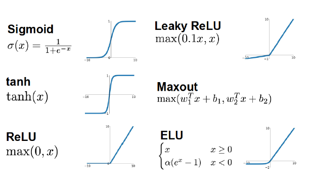
Figure 9.3: Choice of Activation Functions

• Choice of Activation Functions: Some of the Activation Functions discussed in Chapter 7 are shown in Figure 9.3. The general rules in this area are: Avoid Sigmoid and Tanh functions, use ReLu as a default and Leaky ReLU to improve performance, try out MaxOut and ELU on an experimental basis.

• Weight Initialization Rules: Use the Xavier-He initializations as a default (see Chapter 7 for a description).

• Data Pre-Processing and use of Batch Normalization: Data Normalization as a described in Chapter 7 is always advisable and in case of image data, the Centering operation is sufficient. Batch Normalization is a very powerful technique which helps in a vareity of ways, and if you are encountering problems in the training process, then its use is advised.

9.3 How much Data is Needed?

Data is the life blood of Deep Learning models. and sometimes it makes more sense to add to the training dataset rather than use a more sophisticated model. In Chapter 8 we explored the effect of training dataset size and complexity on model performance and its interplay with model capacity, and we summarize the main conclusions here:

• Underfitting: If the model exhibits symptoms of Underfitting, i.e., performance on the training data is poor, then it means that the capacity of the model is not sufficient to correctly classify the training data with a high enough probability of success. In this situation it does not make sense to add more training data, instead the capacity of the model should be increased by adding Hidden Layers or by improving the learning process by using the techniques described in the previous section. If none of these changes result in any improvement, then it points to a problem with the quality of the training data.

• Overfitting: If the model exhibits symptoms of Overfitting, i.e., classification accuracy on the validation data is poor even with low training data error, then it points to lack of sufficient training data. In this situation either more data should be procured or if this is not feasible, then either Regularization should be used to make up for the lack of data (which is the preferred option) or the the capacity of the model should be reduced. It is also possible to expand the training data artificially by using the Data Augmentation techniques discussed in Chapter 8.

A common strategy that is used is to start with a model whose capacity is higher than what may be warranted given the amount of training data, and then add Regularization to avoid Overfitting.

9.4 Tuning Hyper-Parameters

The DLN training process as well as the quality of the model is influenced quite heavily by the choice of hyper-parameters, hence this is an important part of model development. There are two ways in which hyper-parameters are tuned:

• Manual Tuning: The modeler is responsible for searching in the hyper-parameter space to test different parameter combinations.

• Automated Tuning: The hyper-parameter search is automted and is made part of the training algorithm.

We discuss these techniques next.

9.5 Manual Tuning

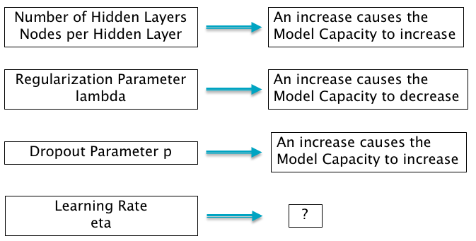
Figure 9.4: Effect of Parameters on Model Capacity

Manual Tuning relies on the modeler’s deep understanding of the DLN model and the training process in order to be able to choose the most appropriate hyper-parameters. A fundamental consideration in manual tuning is the concept of the model capacity, which as the reader may recall from Chapter 8, is the ability of the model handle complex datasets. Different hyper-parameters affect the model capacity differently (see Figure 9.4), in particular:

• Number of Hidden Layers and the number of nodes per Hidden Layer: An increase in these hyper-parameters causes the model capacity to increase.
• Regularization Parameter \(\lambda\): The model capacity increases when the Regularization parameter decreases, since by reducing this parameter we allow the model weight parameters to grow larger.
• Dropout Parameter \(p\): The model capacity decreases when the dropout parameter decreases, since a smaller dropout parameter forces the model to do its job with limited help from other nodes.
• Learning Rate \(\eta\): This is acknowledged to be the most important hyper-parameter. There does not exist a simple relationship between the model capacity and learning rate, but in general the model capacity is maximized if the learning rate is set to the correct value, which may not necessarily be the largest or smallest value.

Among all hyper-parameters, the learning rate is perhaps the most important and is usually chosen first. When the training error is plotted as a function of the of the learning rate, it exhibits a U-shaped curve. If it is set to too high a value, then this can cause the training error to actually increase, while if set too small it not only slows down the training process but can also cause gradient descent to get stuck in a non-optimal point.

In order to tune parameters other than the learning rate, both the training and validation errors need to tracked. Recall that in Figure 8.2 we plotted the training and validation errors as a function of the model capacity, which showed that the validation error in general followed a U-shaped curve as the capacity is varied. Hence the objective of hyper-parameter tuning is to use the rough guidelines in Figure 9.4 to choose the parameters which cause the model capacity to be in the neighborhood of the lowest portion of the validation error curve.

Note that in addition to the hyper-parameter values, the following other factors also influence model capacity:

• The optimization algorithm: For example if optimization gets stuck in non-optimal minima due to a bad initialization, then this restricts the model capacity.

• Regularization: This causes the model capacity to decrease, hence if the system is in a state of underfitting, then adding Regularization won’t help matters much.

Hence model capacity, along with these other factors, determines the Effective Capacity of the model. The objective of hyper-parameter search is to match the effective capacity of the model with the complexity of the task.

9.6 Automated Tuning

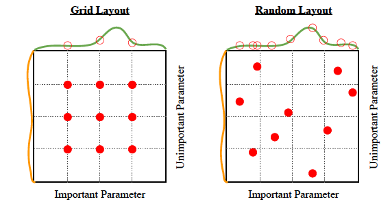
Figure 9.5: Hyper-Parameter Search Techniques

This can be described as a “brute-force” search in the hyper-parameter space in which various combinations are tested using the validation dataset, and the one that has the lowest validation error is chosen. The objective is to automate the model creation process as much as possible, by hiding the details of the hyper-parameter selection process from the user. As shown in Figure 9.5, there are two ways in which this is done:

1. Grid Search: This is an exhaustive search in the parameter space in which all possible combinations are tested, which can get to be very time consuming. Usually works best when there are three or fewer hyper-parameters and for each hyper-parameter the user selects a small finite set of values to explore. The smallest and largest element of each hyper-parameter are chosen, and the remaining values are chosen on the logarithmic scale. For example when choosing learning rates, the range of values to be tested are chosen to be \({0.1, 0.01, 10^{-3}, 10^{-4}, 10^{-5}}\). If the best value is found to be on the edge of set, then a new parameter range should be tested which is also shifted towards to the edge of the original set.

2. Random Search: Instead of doing an exhaustive evaluation all possible hyper-parameter values, Random Search chooses a few random points in the parameter space, see Bergstra and Bengio (2012). This is done by defining a marginal distribution for each hyper-parameter (Bernoulli for binary, multinoulli for discrete, uniform on a log-scale for positive real-valued). For example to choose random learning rates in the range \([10^{-5}, 0.1]\), we would first sample log learning rates from the uniform distribution \(U[-1,-5]\), and then set \[ \lambda = 10^{log\ learning\ rate} \] Random search has been shown to converge much faster to good values of the hyper-parameters, as compared to grid search. The reason for this can be seen in Figure 9.5: If we were restricted to doing nine experiments to find the best set of hyper-parameters, then in Grid Search case we would be limited to searching at three values of each of the two hyper-parameters. However in the Random Search case, we are able to search over a much larger number of possible parameter values, as the figure shows, which results in a faster search.

9.7 Verifying Code Correctness

One of the issues practitioners have with DLN models, is that if the model does not give good results, then it is difficult to pinpoint the source of the error due to the fact that it could have been caused due to a number of factors, including:

• Lack of training data or using test data that comes from a different distribution than the training data
• Wrong choice of model for the given dataset
• Issues in the training process, such as Underfitting, Overfitting, slow Stochastic Gradient iterations etc.
• A bug in the code

So far, in this and the prior two chapters, we discussed ways in which the first three issues could be detected and solved. We now briefly discuss the fourth item, which is the detection of bugs in the DLN code. The following techniques are commonly used in order to accomplish this:

• Check the Loss Function at start of training: The first few iterations of the training process should result in a Loss Function value of approximately \(\log K\), where \(K\) is the number of output classes. This is due to the fact that an un-trained model should assign equal probability to all \(K\) classes. Regularization should be disabled and the Learning Rate set to a small value, such as \(10^{-6}\) while performing this test.

• Fit a small dataset: We can eliminate software bugs as the cause of large training data errors as follows: Cut down the size of the traing dataset to just a few samples, and run the model until the Loss Function goes to zero, at which point the model completely fits the training data. If this does not happen then it points to a bug in the code.

• Verifying Backprop: The implementation of the Backprop algorithm is subject to subtle errors that can nevertheless cause large errors in its output. The value of the derivatives being computed through Backprop can be verified using the method of Finite Differences using the following formula: \[ \frac{\partial\mathcal L}{\partial w_{ij}} \approx \frac{\mathcal L(w_{11},..,w_{ij}+\epsilon,...,w_{mn})-\mathcal L(w_{11},...,w_{ij},...,w_{mn)})}{\epsilon} \] This computation requires two forward passes through the network per derivative.

• Visualize the Results: Instead of relying on just the Loss Function values to verify that the model is working correctly, it is sometimes helpful to look at the output of the model in combination with the corresponding input. This can catch some obvious classification problems that are not obvious from just the Loss Function value.

• Visualize the Mistakes: This involves examining the input data that was mis-classified. Sometimes an examination of the images gives clues about why the mis-classification might have happened. An example than has been often sited is the mis-classification of house numbers found in images from Google Street View, due to the fact that the images were being cropped in such a way that some of the numbers were being left out.

References

Bergstra, James, and Yoshua Bengio. 2012. “Random Search for Hyper-Parameter Optimization.” Journal of Machine Learning Research 13: 281–305. http://dl.acm.org/citation.cfm?id=2188395.