Chapter 10 Deep Learning with R
There are many software packages that offer neural net implementations that may be applied directly. We will survey these as we proceed through the monograph. Our first example will be the use of the R programming language, in which there are many packages for neural networks.
10.1 Breast Cancer Data Set
Our example data set is from the Wisconsin cancer study. We read in the data and remove any rows with missing data. The following code uses the package mlbench that contains this data set. We show the top few lines of the data.
library(mlbench)
data("BreastCancer")

#Clean off rows with missing data
BreastCancer = BreastCancer[which(complete.cases(BreastCancer)==TRUE),]

head(BreastCancer)
## Id Cl.thickness Cell.size Cell.shape Marg.adhesion Epith.c.size
## 1 1000025 5 1 1 1 2
## 2 1002945 5 4 4 5 7
## 3 1015425 3 1 1 1 2
## 4 1016277 6 8 8 1 3
## 5 1017023 4 1 1 3 2
## 6 1017122 8 10 10 8 7
## Bare.nuclei Bl.cromatin Normal.nucleoli Mitoses Class
## 1 1 3 1 1 benign
## 2 10 3 2 1 benign
## 3 2 3 1 1 benign
## 4 4 3 7 1 benign
## 5 1 3 1 1 benign
## 6 10 9 7 1 malignantIn this data set, there are close to 700 samples of tissue taken in biopsies. For each biopsy, nine different characteristics are recorded such as cell thickness, cell size, cell shape. etc. The column names in the data set are as follows.
names(BreastCancer)## [1] "Id" "Cl.thickness" "Cell.size"
## [4] "Cell.shape" "Marg.adhesion" "Epith.c.size"
## [7] "Bare.nuclei" "Bl.cromatin" "Normal.nucleoli"
## [10] "Mitoses" "Class"The last column in the data set is “Class” which is either bening or malignant. The goal of the analysis is to construct a model that learns to decide whether the tumor is malignant or not.
10.2 The deepnet package
The first package in R that we will explore is the deepnet package. Details may be accessed at https://cran.r-project.org/web/packages/deepnet/index.html. We apply the package to the cancer data set as follows. First, we create the dependent variable, and also the feature set of independent variables.
y = as.matrix(BreastCancer[,11])
y[which(y=="benign")] = 0
y[which(y=="malignant")] = 1
y = as.numeric(y)
x = as.numeric(as.matrix(BreastCancer[,2:10]))
x = matrix(as.numeric(x),ncol=9)
We then use the function nn.train from the deepnet package to model the neural network. As can be seen in the program code below, we have 5 nodes in the single hidden layer.
library(deepnet)
nn <- nn.train(x, y, hidden = c(5))
yy = nn.predict(nn, x)
print(head(yy))
## [,1]
## [1,] 0.2823859
## [2,] 0.4459116
## [3,] 0.2975128
## [4,] 0.4505355
## [5,] 0.2971757
## [6,] 0.4796705We take the output of the network and convert it into classes, such that class “0” is benign and class “1” is malignant. We then construct the “confusion matrix” to see how well the model does in-sample. The table function here creates the confusion matrix, which is a tabulation of how many observations that were benign and malignant were correctly classified. This is a handy way of assessing how successful a machine learning model is at classification.
yhat = matrix(0,length(yy),1)
yhat[which(yy > mean(yy))] = 1
yhat[which(yy <= mean(yy))] = 0
cm = table(y,yhat)
print(cm)
## yhat
## y 0 1
## 0 424 20
## 1 5 234We can see that the diagonal of the confusion matrix contains most of the entries, thereby suggesting that the neural net does a very good job of classification. The accuracy may be computed easily as the number of diagnal entries in the confusion matrix divided by the total count of values in the matrix.
print(sum(diag(cm))/sum(cm))## [1] 0.9633968Now that we have seen the model work you can delve into the function nn.train in some more detail to examine the options it allows. The reference manual for the package is available at https://cran.r-project.org/web/packages/deepnet/deepnet.pdf.
10.3 The neuralnet package
For comparison, we try the neuralnet package. The commands are mostly the same. The function in the package is also called neuralnet.
library(neuralnet)
df = data.frame(cbind(x,y))
nn = neuralnet(y~V1+V2+V3+V4+V5+V6+V7+V8+V9,data=df,hidden = 5)
yy = nn$net.result[[1]]
yhat = matrix(0,length(y),1)
yhat[which(yy > mean(yy))] = 1
yhat[which(yy <= mean(yy))] = 0
print(table(y,yhat))
## yhat
## y 0 1
## 0 439 5
## 1 0 239This package also performs very well on this data set. Details about the package and its various functions are available at https://cran.r-project.org/web/packages/neuralnet/index.html.
This package has an interesting function that allows plotting the neural network. Use the function plot() and pass the output object to it, in this case nn. This needs to be run interactively, but here is a sample outpt of the plot.
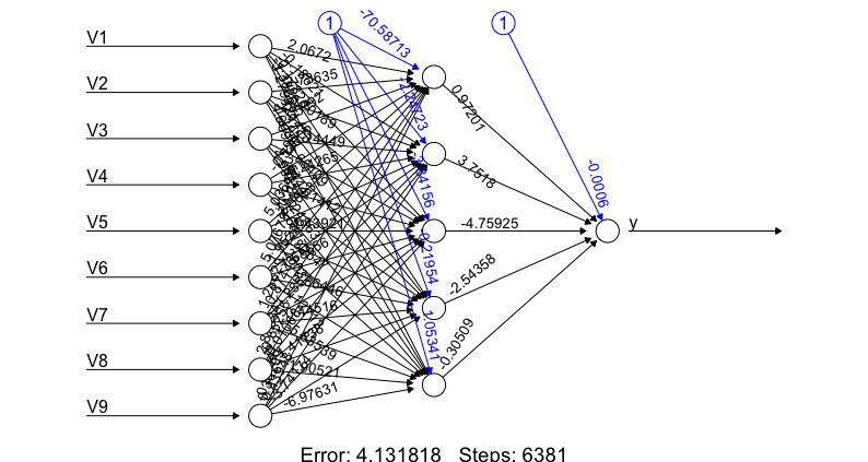
Figure 10.1: Output of the neural net fitting procedure
10.4 Using H2O
The good folks at h2o, see http://www.h2o.ai/, have developed a Java-based version of R, in which they also provide a deep learning network application.
H2O is open source, in-memory, distributed, fast, and provides a scalable machine learning and predictive analytics platform for building machine learning models on big data. H2O’s core code is written in Java. Inside H2O, a Distributed Key/Value store is used to access and reference data, models, objects, etc., across all nodes and machines. The algorithms are implemented in a Map/Reduce framework and utilizes multi-threading. The data is read in parallel and is distributed across the cluster and stored in memory in a columnar format in a compressed way. Therefore, even on a single machine, the deep learning algorithm in H2O will exploit all cores of the CPU in parallel.
Here we start up a server using all cores of the machine, and then use the H2O package’s deep learning toolkit to fit a model.
library(h2o)
localH2O = h2o.init(ip="localhost", port = 54321,
                    startH2O = TRUE, nthreads=-1)

train <- h2o.importFile("BreastCancer.csv")
test <- h2o.importFile("BreastCancer.csv")

y = names(train)[11]
x = names(train)[1:10]

train[,y] = as.factor(train[,y])
test[,y] = as.factor(train[,y])

model = h2o.deeplearning(x=x,
                         y=y,
                         training_frame=train,
                         validation_frame=test,
                         distribution = "multinomial",
                         activation = "RectifierWithDropout",
                         hidden = c(10,10,10,10),
                         input_dropout_ratio = 0.2,
                         l1 = 1e-5,
                         epochs = 50)

print(model)
Model Details:
==============
H2OBinomialModel: deeplearning
Model ID: DeepLearning_model_R_1520814266552_1
Status of Neuron Layers: predicting Class, 2-class classification, multinomial distribution, CrossEntropy loss, 462 weights/biases, 12.5 KB, 34,150 training samples, mini-batch size 1
layer units type dropout l1 l2 mean_rate rate_rms
1 1 10 Input 20.00 %
2 2 10 RectifierDropout 50.00 % 0.000010 0.000000 0.001398 0.000803
3 3 10 RectifierDropout 50.00 % 0.000010 0.000000 0.000994 0.000779
4 4 10 RectifierDropout 50.00 % 0.000010 0.000000 0.000756 0.000385
5 5 10 RectifierDropout 50.00 % 0.000010 0.000000 0.001831 0.003935
6 6 2 Softmax 0.000010 0.000000 0.001651 0.000916
momentum mean_weight weight_rms mean_bias bias_rms
1
2 0.000000 -0.062622 0.378377 0.533913 0.136969
3 0.000000 0.010394 0.343513 0.949866 0.235512
4 0.000000 0.036012 0.326436 0.964657 0.221283
5 0.000000 -0.059503 0.331934 0.784618 0.228269
6 0.000000 0.265010 1.541512 -0.004956 0.121414
H2OBinomialMetrics: deeplearning
** Reported on training data. **
** Metrics reported on full training frame **
MSE: 0.02057362
RMSE: 0.1434351
LogLoss: 0.08568216
Mean Per-Class Error: 0.01994987
AUC: 0.9953871
Gini: 0.9907742
Confusion Matrix (vertical: actual; across: predicted) for F1-optimal threshold:
benign malignant Error Rate
benign 430 14 0.031532 =14/444
malignant 2 237 0.008368 =2/239
Totals 432 251 0.023426 =16/683
Maximum Metrics: Maximum metrics at their respective thresholds
metric threshold value idx
1 max f1 0.330882 0.967347 214
2 max f2 0.253137 0.983471 217
3 max f0point5 0.670479 0.964256 204
4 max accuracy 0.670479 0.976574 204
5 max precision 0.981935 1.000000 0
6 max recall 0.034360 1.000000 241
7 max specificity 0.981935 1.000000 0
8 max absolute_mcc 0.330882 0.949792 214
9 max min_per_class_accuracy 0.608851 0.974895 207
10 max mean_per_class_accuracy 0.330882 0.980050 214
Gains/Lift Table: Extract with `h2o.gainsLift(<model>, <data>)` or `h2o.gainsLift(<model>, valid=<T/F>, xval=<T/F>)`
H2OBinomialMetrics: deeplearning
** Reported on validation data. **
** Metrics reported on full validation frame **
MSE: 0.02057362
RMSE: 0.1434351
LogLoss: 0.08568216
Mean Per-Class Error: 0.01994987
AUC: 0.9953871
Gini: 0.9907742
Confusion Matrix (vertical: actual; across: predicted) for F1-optimal threshold:
benign malignant Error Rate
benign 430 14 0.031532 =14/444
malignant 2 237 0.008368 =2/239
Totals 432 251 0.023426 =16/683
Maximum Metrics: Maximum metrics at their respective thresholds
metric threshold value idx
1 max f1 0.330882 0.967347 216
2 max f2 0.253137 0.983471 219
3 max f0point5 0.670479 0.964256 206
4 max accuracy 0.670479 0.976574 206
5 max precision 0.981935 1.000000 0
6 max recall 0.034360 1.000000 243
7 max specificity 0.981935 1.000000 0
8 max absolute_mcc 0.330882 0.949792 216
9 max min_per_class_accuracy 0.608851 0.974895 209
10 max mean_per_class_accuracy 0.330882 0.980050 216
Gains/Lift Table: Extract with `h2o.gainsLift(<model>, <data>)` or `h2o.gainsLift(<model>, valid=<T/F>, xval=<T/F>)`The h2o deep learning package does very well. The error rate may be seen from the confusion matrix to be very low. We also note that H2O may be used to run analyses other than deep learning in R as well, as many other functions are provided, using almost identical syntax to R. See the documentation at H2O for more details: http://docs.h2o.ai/h2o/latest-stable/index.html
10.5 Image Recognition
As a second case, we use the MNIST dataset, replicating an example from the H2O deep learning manual. This character (numerical digits) recognition example is a classic one in machine learning. First read in the data.
library(h2o)
localH2O = h2o.init(ip="localhost", port = 54321,
                    startH2O = TRUE)

## Import MNIST CSV as H2O
train <- h2o.importFile("train.csv")
test <- h2o.importFile("test.csv")

print(dim(train))
print(dim(test))
[1] 60000 785
[1] 10000 785As we see there are 70,000 observations in the data set with each example containing all the 784 pixels in each image, defining the character. This suggests a very large input data set. Now, we have a much larger parameter space that needs to be fit by the deep learning net. We use a three hidden layer model, with each hidden layer having 10 nodes.
y <- "C785"
x <- setdiff(names(train), y)
train[,y] <- as.factor(train[,y])
test[,y] <- as.factor(test[,y])

# Train a Deep Learning model and validate on a test set
model <- h2o.deeplearning(x = x,
                          y = y,
                          training_frame = train,
                          validation_frame = test,
                          distribution = "multinomial",
                          activation = "RectifierWithDropout",
                          hidden = c(10,10,10),
                          input_dropout_ratio = 0.2,
                          l1 = 1e-5,
epochs = 20)print(model)Model Details:
==============
H2OMultinomialModel: deeplearning
Model ID: DeepLearning_model_R_1520814266552_6
Status of Neuron Layers: predicting C785, 10-class classification, multinomial distribution, CrossEntropy loss, 7,510 weights/biases, 302.2 KB, 1,200,366 training samples, mini-batch size 1
layer units type dropout l1 l2 mean_rate rate_rms
1 1 717 Input 20.00 %
2 2 10 RectifierDropout 50.00 % 0.000010 0.000000 0.025009 0.063560
3 3 10 RectifierDropout 50.00 % 0.000010 0.000000 0.000087 0.000078
4 4 10 RectifierDropout 50.00 % 0.000010 0.000000 0.000265 0.000210
5 5 10 Softmax 0.000010 0.000000 0.002039 0.001804
momentum mean_weight weight_rms mean_bias bias_rms
1
2 0.000000 0.041638 0.198974 0.056699 0.585353
3 0.000000 -0.001518 0.212653 0.907466 0.234638
4 0.000000 -0.072600 0.377217 0.818470 0.442677
5 0.000000 -1.384572 1.744110 -3.993273 0.785979
H2OMultinomialMetrics: deeplearning
** Reported on training data. **
** Metrics reported on temporary training frame with 10082 samples **
Training Set Metrics:
=====================
MSE: (Extract with `h2o.mse`) 0.3571086
RMSE: (Extract with `h2o.rmse`) 0.5975856
Logloss: (Extract with `h2o.logloss`) 0.9939315
Mean Per-Class Error: 0.2470953
Confusion Matrix: Extract with `h2o.confusionMatrix(<model>,train = TRUE)`)
=========================================================================
Confusion Matrix: Row labels: Actual class; Column labels: Predicted class
0 1 2 3 4 5 6 7 8 9 Error Rate
0 810 0 1 2 0 138 6 0 4 0 0.1571 = 151 / 961
1 0 924 3 2 3 30 13 0 148 3 0.1794 = 202 / 1,126
2 0 23 621 34 9 38 183 0 99 4 0.3858 = 390 / 1,011
3 4 0 9 636 2 373 11 1 29 15 0.4111 = 444 / 1,080
4 0 2 0 0 924 42 15 0 7 23 0.0879 = 89 / 1,013
5 11 2 2 26 6 822 10 1 14 4 0.0846 = 76 / 898
6 2 8 3 0 3 70 845 0 9 0 0.1011 = 95 / 940
7 7 0 3 93 35 19 8 676 7 217 0.3653 = 389 / 1,065
8 0 5 8 25 3 240 8 0 699 2 0.2939 = 291 / 990
9 1 1 2 17 336 36 3 5 3 594 0.4048 = 404 / 998
Totals 835 965 652 835 1321 1808 1102 683 1019 862 0.2510 = 2,531 / 10,082
Hit Ratio Table: Extract with `h2o.hit_ratio_table(<model>,train = TRUE)`
=======================================================================
Top-10 Hit Ratios:
k hit_ratio
1 1 0.748958
2 2 0.903591
3 3 0.948423
4 4 0.967169
5 5 0.976592
6 6 0.984527
7 7 0.990081
8 8 0.994247
9 9 0.997818
10 10 1.000000
H2OMultinomialMetrics: deeplearning
** Reported on validation data. **
** Metrics reported on full validation frame **
Validation Set Metrics:
=====================
Extract validation frame with `h2o.getFrame("RTMP_sid_8178_8")`
MSE: (Extract with `h2o.mse`) 0.3585186
RMSE: (Extract with `h2o.rmse`) 0.5987642
Logloss: (Extract with `h2o.logloss`) 0.9993684
Mean Per-Class Error: 0.2486848
Confusion Matrix: Extract with `h2o.confusionMatrix(<model>,valid = TRUE)`)
=========================================================================
Confusion Matrix: Row labels: Actual class; Column labels: Predicted class
0 1 2 3 4 5 6 7 8 9 Error Rate
0 867 0 0 3 1 104 5 0 0 0 0.1153 = 113 / 980
1 0 925 2 2 0 14 5 0 187 0 0.1850 = 210 / 1,135
2 2 30 657 30 15 50 139 2 107 0 0.3634 = 375 / 1,032
3 1 0 9 574 2 378 8 2 28 8 0.4317 = 436 / 1,010
4 0 0 2 3 926 24 16 0 4 7 0.0570 = 56 / 982
5 11 0 1 27 8 806 13 1 20 5 0.0964 = 86 / 892
6 4 5 2 0 5 71 867 0 4 0 0.0950 = 91 / 958
7 6 0 8 99 39 18 7 644 17 190 0.3735 = 384 / 1,028
8 4 7 9 29 4 220 8 0 684 9 0.2977 = 290 / 974
9 2 0 0 14 403 47 3 2 5 533 0.4718 = 476 / 1,009
Totals 897 967 690 781 1403 1732 1071 651 1056 752 0.2517 = 2,517 / 10,000
Hit Ratio Table: Extract with `h2o.hit_ratio_table(<model>,valid = TRUE)`
=======================================================================
Top-10 Hit Ratios:
k hit_ratio
1 1 0.748300
2 2 0.903200
3 3 0.946200
4 4 0.966000
5 5 0.977300
6 6 0.984800
7 7 0.989300
8 8 0.993600
9 9 0.997800
10 10 1.000000The mean error is much higher here, around a third. It looks like the highest error arises from the DLN mistaking the number “8” for the number “1”. It also seems to confuse the number “3” for the number “5”. However, it appears to do best in identifying the numbers “3” and “7”.
We repeat the model with a deeper net with more nodes to see if accuracy increases.
y <- "C785"
x <- setdiff(names(train), y)
train[,y] <- as.factor(train[,y])
test[,y] <- as.factor(test[,y])

# Train a Deep Learning model and validate on a test set
model <- h2o.deeplearning(x = x,
                          y = y,
                          training_frame = train,
                          validation_frame = test,
                          distribution = "multinomial",
                          activation = "RectifierWithDropout",
                          hidden = c(50,50,50,50,50),
                          input_dropout_ratio = 0.2,
                          l1 = 1e-5,
epochs = 20)print(model)Model Details:
==============
H2OMultinomialModel: deeplearning
Model ID: DeepLearning_model_R_1520808969376_7
Status of Neuron Layers: predicting C785, 10-class classification, multinomial distribution, CrossEntropy loss, 46,610 weights/biases, 762.1 KB, 1,213,670 training samples, mini-batch size 1
layer units type dropout l1 l2 mean_rate rate_rms momentum mean_weight
1 1 717 Input 20.00 %
2 2 50 RectifierDropout 50.00 % 0.000010 0.000000 0.033349 0.086208 0.000000 0.045794
3 3 50 RectifierDropout 50.00 % 0.000010 0.000000 0.000306 0.000142 0.000000 -0.045147
4 4 50 RectifierDropout 50.00 % 0.000010 0.000000 0.000560 0.000327 0.000000 -0.043226
5 5 50 RectifierDropout 50.00 % 0.000010 0.000000 0.000729 0.000397 0.000000 -0.038671
6 6 50 RectifierDropout 50.00 % 0.000010 0.000000 0.000782 0.000399 0.000000 -0.054582
7 7 10 Softmax 0.000010 0.000000 0.004216 0.004104 0.000000 -0.626657
weight_rms mean_bias bias_rms
1
2 0.122829 -0.195569 0.319780
3 0.155798 0.832219 0.187684
4 0.164139 0.807165 0.206030
5 0.157497 0.774994 0.248565
6 0.154222 0.657222 0.258284
7 1.017226 -3.836859 0.773292
H2OMultinomialMetrics: deeplearning
** Reported on training data. **
** Metrics reported on temporary training frame with 10097 samples **
Training Set Metrics:
=====================
MSE: (Extract with `h2o.mse`) 0.1109938732
RMSE: (Extract with `h2o.rmse`) 0.33315743
Logloss: (Extract with `h2o.logloss`) 0.3742232893
Mean Per-Class Error: 0.09170121783
Confusion Matrix: Extract with `h2o.confusionMatrix(<model>,train = TRUE)`)
=========================================================================
Confusion Matrix: Row labels: Actual class; Column labels: Predicted class
0 1 2 3 4 5 6 7 8 9 Error Rate
0 969 0 2 0 0 8 15 4 9 1 0.0387 = 39 / 1,008
1 0 1048 17 3 1 0 0 2 6 3 0.0296 = 32 / 1,080
2 4 4 930 11 1 1 8 7 37 5 0.0774 = 78 / 1,008
3 2 3 15 884 0 11 3 17 64 7 0.1213 = 122 / 1,006
4 0 3 2 0 855 1 2 0 4 97 0.1131 = 109 / 964
5 7 0 15 13 3 649 3 3 206 5 0.2821 = 255 / 904
6 11 1 14 0 4 12 967 0 5 2 0.0482 = 49 / 1,016
7 2 9 4 14 3 0 0 1006 2 36 0.0651 = 70 / 1,076
8 2 17 18 7 2 3 3 1 958 13 0.0645 = 66 / 1,024
9 3 6 0 10 10 1 1 30 17 933 0.0772 = 78 / 1,011
Totals 1000 1091 1017 942 879 686 1002 1070 1308 1102 0.0889 = 898 / 10,097
Hit Ratio Table: Extract with `h2o.hit_ratio_table(<model>,train = TRUE)`
=======================================================================
Top-10 Hit Ratios:
k hit_ratio
1 1 0.911063
2 2 0.965336
3 3 0.979697
4 4 0.986729
5 5 0.990393
6 6 0.993661
7 7 0.996138
8 8 0.998415
9 9 0.999604
10 10 1.000000
H2OMultinomialMetrics: deeplearning
** Reported on validation data. **
** Metrics reported on full validation frame **
Validation Set Metrics:
=====================
Extract validation frame with `h2o.getFrame("RTMP_sid_9f65_10")`
MSE: (Extract with `h2o.mse`) 0.110646279
RMSE: (Extract with `h2o.rmse`) 0.3326353544
Logloss: (Extract with `h2o.logloss`) 0.3800417831
Mean Per-Class Error: 0.0919470552
Confusion Matrix: Extract with `h2o.confusionMatrix(<model>,valid = TRUE)`)
=========================================================================
Confusion Matrix: Row labels: Actual class; Column labels: Predicted class
0 1 2 3 4 5 6 7 8 9 Error Rate
0 945 0 1 1 0 11 16 3 3 0 0.0357 = 35 / 980
1 0 1114 10 1 0 0 3 0 5 2 0.0185 = 21 / 1,135
2 8 1 955 9 4 1 8 7 37 2 0.0746 = 77 / 1,032
3 0 3 19 890 0 10 0 17 68 3 0.1188 = 120 / 1,010
4 0 0 10 0 846 1 11 3 5 106 0.1385 = 136 / 982
5 6 0 14 19 2 658 1 7 173 12 0.2623 = 234 / 892
6 14 2 10 0 8 10 909 0 5 0 0.0511 = 49 / 958
7 0 8 16 15 1 1 1 941 2 43 0.0846 = 87 / 1,028
8 4 7 19 6 6 6 3 8 906 9 0.0698 = 68 / 974
9 4 7 2 7 9 4 1 13 19 943 0.0654 = 66 / 1,009
Totals 981 1142 1056 948 876 702 953 999 1223 1120 0.0893 = 893 / 10,000
Hit Ratio Table: Extract with `h2o.hit_ratio_table(<model>,valid = TRUE)`
=======================================================================
Top-10 Hit Ratios:
k hit_ratio
1 1 0.910700
2 2 0.961900
3 3 0.975400
4 4 0.984400
5 5 0.990700
6 6 0.994200
7 7 0.996000
8 8 0.998100
9 9 0.999100
10 10 1.000000In fact now the error rate is greatly reduced. It is useful to assess whether the improvement comes from more nodes in each layer or more hidden layers.
y <- "C785"
x <- setdiff(names(train), y)
train[,y] <- as.factor(train[,y])
test[,y] <- as.factor(test[,y])

# Train a Deep Learning model and validate on a test set
model <- h2o.deeplearning(x = x,
                          y = y,
                          training_frame = train,
                          validation_frame = test,
                          distribution = "multinomial",
                          activation = "RectifierWithDropout",
                          hidden = c(100,100,100),
                          input_dropout_ratio = 0.2,
                          l1 = 1e-5,
epochs = 20)print(model)Model Details:
==============
H2OMultinomialModel: deeplearning
Model ID: DeepLearning_model_R_1520808969376_9
Status of Neuron Layers: predicting C785, 10-class classification, multinomial distribution, CrossEntropy loss, 93,010 weights/biases, 1.3 MB, 1,224,061 training samples, mini-batch size 1
layer units type dropout l1 l2 mean_rate rate_rms momentum mean_weight
1 1 717 Input 20.00 %
2 2 100 RectifierDropout 50.00 % 0.000010 0.000000 0.048155 0.113535 0.000000 0.036710
3 3 100 RectifierDropout 50.00 % 0.000010 0.000000 0.000400 0.000184 0.000000 -0.036035
4 4 100 RectifierDropout 50.00 % 0.000010 0.000000 0.000833 0.000436 0.000000 -0.029517
5 5 10 Softmax 0.000010 0.000000 0.007210 0.019309 0.000000 -0.521292
weight_rms mean_bias bias_rms
1
2 0.111724 -0.351463 0.255260
3 0.099199 0.820070 0.119388
4 0.103166 0.509412 0.127704
5 0.747221 -3.036467 0.279808
H2OMultinomialMetrics: deeplearning
** Reported on training data. **
** Metrics reported on temporary training frame with 9905 samples **
Training Set Metrics:
=====================
MSE: (Extract with `h2o.mse`) 0.03222117368
RMSE: (Extract with `h2o.rmse`) 0.1795025729
Logloss: (Extract with `h2o.logloss`) 0.1149316416
Mean Per-Class Error: 0.03563532983
Confusion Matrix: Extract with `h2o.confusionMatrix(<model>,train = TRUE)`)
=========================================================================
Confusion Matrix: Row labels: Actual class; Column labels: Predicted class
0 1 2 3 4 5 6 7 8 9 Error Rate
0 998 0 4 1 2 1 1 0 2 0 0.0109 = 11 / 1,009
1 0 1086 9 5 0 0 2 5 6 0 0.0243 = 27 / 1,113
2 4 0 926 3 3 0 3 6 3 0 0.0232 = 22 / 948
3 0 0 16 993 0 11 1 12 2 2 0.0424 = 44 / 1,037
4 1 3 8 0 902 0 6 1 6 23 0.0505 = 48 / 950
5 4 0 0 14 0 832 13 3 2 2 0.0437 = 38 / 870
6 4 2 8 0 2 7 988 0 4 0 0.0266 = 27 / 1,015
7 3 2 6 1 2 2 1 984 1 2 0.0199 = 20 / 1,004
8 2 1 6 6 3 13 6 2 923 1 0.0415 = 40 / 963
9 5 0 3 13 12 5 0 22 13 923 0.0733 = 73 / 996
Totals 1021 1094 986 1036 926 871 1021 1035 962 953 0.0353 = 350 / 9,905
Hit Ratio Table: Extract with `h2o.hit_ratio_table(<model>,train = TRUE)`
=======================================================================
Top-10 Hit Ratios:
k hit_ratio
1 1 0.964664
2 2 0.988895
3 3 0.995558
4 4 0.997577
5 5 0.998789
6 6 0.999091
7 7 0.999495
8 8 0.999798
9 9 1.000000
10 10 1.000000
H2OMultinomialMetrics: deeplearning
** Reported on validation data. **
** Metrics reported on full validation frame **
Validation Set Metrics:
=====================
Extract validation frame with `h2o.getFrame("RTMP_sid_9f65_14")`
MSE: (Extract with `h2o.mse`) 0.03617073617
RMSE: (Extract with `h2o.rmse`) 0.1901860567
Logloss: (Extract with `h2o.logloss`) 0.1443472174
Mean Per-Class Error: 0.03971753401
Confusion Matrix: Extract with `h2o.confusionMatrix(<model>,valid = TRUE)`)
=========================================================================
Confusion Matrix: Row labels: Actual class; Column labels: Predicted class
0 1 2 3 4 5 6 7 8 9 Error Rate
0 967 0 1 1 0 3 4 2 1 1 0.0133 = 13 / 980
1 0 1114 7 2 0 0 4 1 7 0 0.0185 = 21 / 1,135
2 8 1 990 6 5 1 7 8 6 0 0.0407 = 42 / 1,032
3 0 0 11 979 0 6 0 7 7 0 0.0307 = 31 / 1,010
4 1 1 5 0 926 3 10 5 4 27 0.0570 = 56 / 982
5 3 0 3 17 2 851 7 1 5 3 0.0460 = 41 / 892
6 10 4 4 0 4 6 927 0 3 0 0.0324 = 31 / 958
7 2 6 19 3 0 0 0 992 0 6 0.0350 = 36 / 1,028
8 5 2 7 5 3 17 2 6 925 2 0.0503 = 49 / 974
9 5 4 2 9 10 11 0 24 9 935 0.0733 = 74 / 1,009
Totals 1001 1132 1049 1022 950 898 961 1046 967 974 0.0394 = 394 / 10,000
Hit Ratio Table: Extract with `h2o.hit_ratio_table(<model>,valid = TRUE)`
=======================================================================
Top-10 Hit Ratios:
k hit_ratio
1 1 0.960600
2 2 0.983200
3 3 0.992200
4 4 0.995700
5 5 0.997800
6 6 0.998600
7 7 0.999300
8 8 0.999800
9 9 1.000000
10 10 1.000000The error rate is now extremeley low, so the number of nodes per hidden layer seems to matter more. However, we do need to note that this is more art than science, and we should make sure that we try various different DLNs before settling on the final one for our application.
10.6 Using MXNET
MXNET is another excellent library for Deep Learning. It is remarkable in that is has been developed mostly by graduate students and academics from several universities such as CMU, NYU, NUS, and MIT, among many others. MXNET stands for “mix” and “maximize” and runs on many different hardware platforms, and uses CPUs and GPUs. It can also run in distributed mode as well. For the main page of this open source project, see http://mxnet.io/.
MXNET may be used from more programming languages than other deep learning frameworks. It supports C++, R, Python, Julia, Scala, Perl, Matlab, Go, and Javascript. It has CUDA support, and also includes specialized neural nets such as convolutional neural nets (CNNs), recurrent neural nets (RNNs), restricted Boltzmann machines (RBMs), and deep belief networks (DBNs).
MXNET may be run in the cloud using the Amazon AWS platform, on which there are several deep learning virtual machines available that run the library. See: https://aws.amazon.com/mxnet/
We illustrate the use of MXNET using the breast cancer data set. As before, we set up the data first.
library(mxnet)
data("BreastCancer")
BreastCancer = BreastCancer[which(complete.cases(BreastCancer)==TRUE),]

y = as.matrix(BreastCancer[,11])
y[which(y=="benign")] = 0
y[which(y=="malignant")] = 1
y = as.numeric(y)
x = as.numeric(as.matrix(BreastCancer[,2:10]))
x = matrix(as.numeric(x),ncol=9)

train.x = x
train.y = y
test.x = x
test.y = y

mx.set.seed(0)
model <- mx.mlp(train.x, train.y, hidden_node=c(5,5), out_node=2, out_activation="softmax", num.round=20, array.batch.size=32, learning.rate=0.07, momentum=0.9, eval.metric=mx.metric.accuracy)

preds = predict(model, test.x)
## Auto detect layout of input matrix, use rowmajor..
pred.label = max.col(t(preds))-1
table(pred.label, test.y)
The results of the training run are as follows.
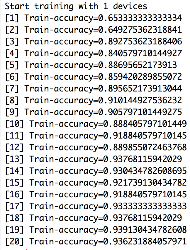
Figure 10.2: Training epochs for the cancer data set
The results of the validation run are as follows.
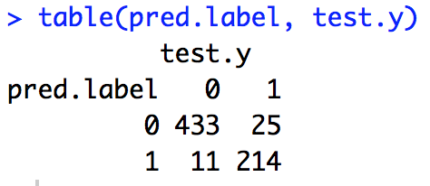
Figure 10.3: Testing confusion matrix for the cancer data set
And, for a second example for MXNET, we revisit the standard MNIST data set. (We do not always run this model, as it seems to be very slow om CPUs.)
## Import MNIST CSV
train <- read.csv("train.csv",header = TRUE)
test <- read.csv("test.csv",header = TRUE)
train = data.matrix(train)
test = data.matrix(test)

train.x = train[,1:784]/255  #Normalize the data
train.y = train[,785]
test.x = test[,1:784]/255
test.y = test[,785]

mx.set.seed(0)
model <- mx.mlp(train.x, train.y, hidden_node=c(100,100,100), out_node=10, out_activation="softmax", num.round=10, array.batch.size=32, learning.rate=0.05, eval.metric=mx.metric.accuracy, optimizer='sgd')

preds = predict(model, test.x)
## Auto detect layout of input matrix, use rowmajor..
pred.label = max.col(t(preds))-1
cm = table(pred.label, test.y)
print(cm)
acc = sum(diag(cm))/sum(cm)
print(acc)
The results of the training run are as follows.
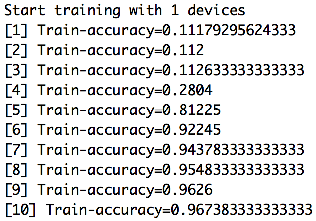
Figure 10.4: Training epochs for the MNIST data set
The results of the validation run are as follows.
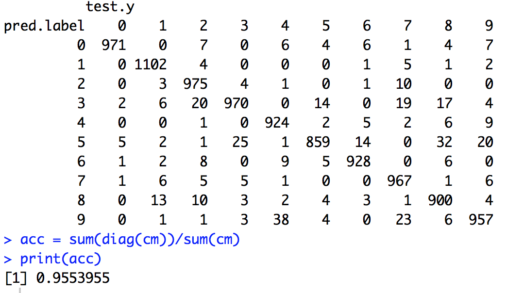
Figure 10.5: Testing confusion matrix for the MNIST data set
10.7 Using TensorFlow
TensorFlow (from Google, we will refer to it by short form “TF”) is an open source deep neural net framework, based on a graphical model. It is more than just a neural net platform, and supports numerical computing based on data flow graphs. Data may be represented in \(n\)-dimensional structures like vectors and matrices, or higher-dimensional tensors. Because these mathematical objects are folded into a data flow graph for computation, the moniker for this software library is an obvious one.
The computations for deep learning nets involve tensor computations, which are known to be implemented more efficiently on GPUs than CPUs. Therefore like other deep learning libraries, TensorFlow may be implemented on CPUs and GPUs. The generality and speed of the TensorFlow software, ease of installation, its documentation and examples, and runnability on multiple platforms has made TensorFlow the most popular deep learning toolkit today. (Opinions on this may, of course, differ.) There is a wealth of tutorial material on TF of very high quality that you may refer to here: https://www.tensorflow.org/tutorials/.
Rather than run TF natively, it is often easier to use it through an easy to use interface program. One of the most popular high-level APIs is Keras. See: https://keras.io/. The site contains several examples, which make it easy to get up and running. Though originally written in Python, Keras has been extended to R via the KerasR package.
We will rework the earlier examples to exemplify how easy it is to implement TF in R using Keras. We need two specific libraries in R to run TF. One is TF itself. The other is Keras (https://keras.io/). So, we go ahead and load up these two libraries, assuming of course, that you have installed them already.
library(tensorflow)
library(kerasR)
10.7.1 Detecting Cancer
As before, we read in the breast cancer data set. There is nothing different here, except for the last line in the next code block, where we convert the tags (benign, malignant) in the data set to “one-hot encoding” using the to_categorial function. What is one-hot encoding, you may ask? Instead of a single vector of 1s (malignant) and 0s (benign), we describe the bivariate dependent variable as a two-column matrix, where the first column contains a 1 if the cell is benign and the second column a 1 if the cell is malignant, for each row of the data set. This is because TF/Keras requires this format as input, to facilitate tensor calculations.
tf_train <- read.csv("BreastCancer.csv")
tf_test <- read.csv("BreastCancer.csv")

X_train = as.matrix(tf_train[,2:10])
X_test = as.matrix(tf_test[,2:10])
y_train = as.matrix(tf_train[,11])
y_test = as.matrix(tf_test[,11])

idx = which(y_train=="benign"); y_train[idx]=0; y_train[-idx]=1; y_train=as.integer(y_train)
idx = which(y_test=="benign"); y_test[idx]=0; y_test[-idx]=1; y_test=as.integer(y_test)

Y_train <- to_categorical(y_train,2)
10.7.2 Set up and compile the model
TensorFlow is structured in a manner where one describes the neural net first, layer by layer. Unlike the other packages we have seen earlier, in TF, we do not have a single function that is called, which generates the deep learning net, and runs the model. Here, we first describe for each layer in the neural net, the number of nodes, the type of activation function, and any other hyperparameters needed in the model fitting stage, such as the extent of dropout for example. In the output layer we also state the nature of the activation function, such as sigmoid or softmax. And then, we specify a compile function which describes the loss function that will be minimized, along with the minimization algorithm. At this point in the program specification, the model is not actually run. See below for the code block that builds up the deep learning network.
n_units = 512

mod <- Sequential()
mod$add(Dense(units = n_units, input_shape = dim(X_train)[2]))
mod$add(LeakyReLU())
mod$add(Dropout(0.25))

mod$add(Dense(units = n_units))
mod$add(LeakyReLU())
mod$add(Dropout(0.25))

mod$add(Dense(units = n_units))
mod$add(LeakyReLU())
mod$add(Dropout(0.25))

mod$add(Dense(units = n_units))
mod$add(LeakyReLU())
mod$add(Dropout(0.25))

mod$add(Dense(units = n_units))
mod$add(LeakyReLU())
mod$add(Dropout(0.25))

mod$add(Dense(2))
mod$add(Activation("softmax"))

keras_compile(mod, loss = 'categorical_crossentropy', optimizer = RMSprop())
10.7.3 Fit the deep learning net
We are now ready to fit the model. In order to do so, we specify the number of epochs to be run. Recall that running too many epochs will result in overfitting the model in-sample, and result in poor performance out-of-sample. So we try to run only a few epochs here. The number of epochs depends on the nature of the problem. For the example problems here, we need very few epochs. For image recognition problems, or natural language problems, we usually end up needing many more.
We also specify the batch size, as this is needed for stochastic batch gradient descent, discussed earlier in Chapter 7. When we run the code below, we see TF running one epoch at a time. The accuracy and loss function value are reported for each epoch.
keras_fit(mod, X_train, Y_train, batch_size = 32, epochs = 15, verbose = 2, validation_split = 1.0)Epoch 1/15
2018-03-11 17:14:53.534398: W tensorflow/core/platform/cpu_feature_guard.cc:45] The TensorFlow library wasn't compiled to use SSE4.2 instructions, but these are available on your machine and could speed up CPU computations.
2018-03-11 17:14:53.534428: W tensorflow/core/platform/cpu_feature_guard.cc:45] The TensorFlow library wasn't compiled to use AVX instructions, but these are available on your machine and could speed up CPU computations.
2018-03-11 17:14:53.534448: W tensorflow/core/platform/cpu_feature_guard.cc:45] The TensorFlow library wasn't compiled to use AVX2 instructions, but these are available on your machine and could speed up CPU computations.
2018-03-11 17:14:53.534453: W tensorflow/core/platform/cpu_feature_guard.cc:45] The TensorFlow library wasn't compiled to use FMA instructions, but these are available on your machine and could speed up CPU computations.
0s - loss: 5.1941
Epoch 2/15
0s - loss: 0.6029
Epoch 3/15
0s - loss: 0.3213
Epoch 4/15
0s - loss: 0.2806
Epoch 5/15
0s - loss: 0.2619
Epoch 6/15
0s - loss: 0.2079
Epoch 7/15
0s - loss: 0.1853
Epoch 8/15
0s - loss: 0.1550
Epoch 9/15
0s - loss: 0.1366
Epoch 10/15
0s - loss: 0.1259
Epoch 11/15
0s - loss: 0.1208
Epoch 12/15
0s - loss: 0.1115
Epoch 13/15
0s - loss: 0.0999
Epoch 14/15
0s - loss: 0.1423
Epoch 15/15
0s - loss: 0.0945Once the model is fit, we then check accuracy and predictions.
#Validation
Y_test_hat <- keras_predict_classes(mod, X_test)
table(y_test, Y_test_hat)
print(c("Mean validation accuracy = ",mean(y_test == Y_test_hat)))
32/683 [>.............................] - ETA: 1s
Y_test_hat
y_test 0 1
0 435 9
1 8 231
[1] "Mean validation accuracy = " "0.97510980966325"10.7.4 The MNIST Example: The “Hello World” of Deep Learning
We now revisit the digit recognition problem from earlier to see how to implement it in TF. Load in the MNIST data. Example taken from: https://cran.r-project.org/web/packages/kerasR/vignettes/introduction.html
library(data.table)
train = as.data.frame(fread("train.csv"))
test = as.data.frame(fread("test.csv"))
#mnist <- load_mnist()
X_train <- as.matrix(train[,-1])
Y_train <- as.matrix(train[,785])
X_test <- as.matrix(test[,-1])
Y_test <- as.matrix(test[,785])
dim(X_train)
[1] 60000 784Notice that the training dataset is in the form of 3d tensors, of size \(60,000 \times 28 \times 28\). This is where the “tensor” moniker comes from, and the “flow” part comes from the internal representation of the calculations on a flow network from input to eventual output.
10.7.5 Normalization
Now we normalize the values, which are pixel intensities ranging in \((0,255)\).
X_train <- array(X_train, dim = c(dim(X_train)[1], prod(dim(X_train)[-1]))) / 255
X_test <- array(X_test, dim = c(dim(X_test)[1], prod(dim(X_test)[-1]))) / 255
And then, convert the \(Y\) variable to categorical (one-hot encoding).
Y_train <- to_categorical(Y_train, num_classes=10)10.7.6 Construct the Deep Learning Net
Now create the model in Keras.
n_units = 100  ## tf example is 512, acc=95%, with 100, acc=96%

mod <- Sequential()
mod$add(Dense(units = n_units, input_shape = dim(X_train)[2]))
mod$add(LeakyReLU())
mod$add(Dropout(0.25))

mod$add(Dense(units = n_units))
mod$add(LeakyReLU())
mod$add(Dropout(0.25))

mod$add(Dense(units = n_units))
mod$add(LeakyReLU())
mod$add(Dropout(0.25))

mod$add(Dense(10))
mod$add(Activation("softmax"))
10.7.7 Compilation
Then, compile the model.
keras_compile(mod, loss = 'categorical_crossentropy', optimizer = RMSprop())10.7.8 Fit the Model
Now run the model to get a fitted deep learning network.
keras_fit(mod, X_train, Y_train, batch_size = 32, epochs = 5, verbose = 2, validation_split = 0.1)Train on 54000 samples, validate on 6000 samples
Epoch 1/5
4s - loss: 0.4112 - val_loss: 0.2211
Epoch 2/5
4s - loss: 0.2710 - val_loss: 0.1910
Epoch 3/5
4s - loss: 0.2429 - val_loss: 0.1683
Epoch 4/5
4s - loss: 0.2283 - val_loss: 0.1712
Epoch 5/5
4s - loss: 0.2217 - val_loss: 0.148210.7.9 Quality of Fit
Check accuracy and predictions.
Y_test_hat <- keras_predict_classes(mod, X_test)
table(Y_test, Y_test_hat)
mean(Y_test == as.matrix(Y_test_hat))
8192/10000 [=======================>......] - ETA: 0s
Y_test_hat
Y_test 0 1 2 3 4 5 6 7 8 9
0 970 0 0 1 0 3 2 2 2 0
1 0 1120 4 3 0 1 3 0 4 0
2 7 1 980 7 4 1 6 7 18 1
3 0 0 12 962 0 16 0 7 8 5
4 1 1 3 0 915 0 10 2 12 38
5 3 1 0 8 1 857 9 2 6 5
6 11 3 1 0 4 8 922 1 8 0
7 1 12 17 13 1 0 0 957 4 23
8 7 2 3 6 3 7 7 3 930 6
9 4 5 0 8 4 2 0 3 4 979
[1] 0.959210.8 Using TensorFlow with keras (instead of kerasR)
There are two packages available for the front end of TensorFlow. One we have seen, is kerasR and in this section we will use keras. In R the usage is slightly different, and the reader may prefer one versus the other. Technically, there is no difference. The main difference is in the way we write code for the two different alternatives. The previous approach was in a functional programming style, whereas this one is more object-oriented.
We first load up the library called keras. And we initialize the fully-connected feed-forward neural net model. (Since we will be using pipes, we also load up the magrittr package.)
library(magrittr)
library(keras)
model <- keras_model_sequential()
Next, we define the deep learning model.
n_units = 100
model %>%
  layer_dense(units = n_units,
              activation = 'relu',
              input_shape = dim(X_train)[2]) %>%
  layer_dropout(rate = 0.25) %>%
  layer_dense(units = n_units, activation = 'relu') %>%
  layer_dropout(rate = 0.25) %>%
  layer_dense(units = n_units, activation = 'relu') %>%
  layer_dropout(rate = 0.25) %>%
  layer_dense(units = 10, activation = 'softmax')
Now, compile the model.
model %>% compile(
  loss = 'categorical_crossentropy',
  optimizer = optimizer_rmsprop(),
  metrics = c('accuracy')
)
Finally, fit the model. We will run just 5 epochs.
model %>% fit(
  X_train, Y_train,
  epochs = 5, batch_size = 32, verbose = 1,
  validation_split = 0.1
)
Train on 54000 samples, validate on 6000 samples
Epoch 1/5
54000/54000 [==============================] - 3s - loss: 0.4199 - acc: 0.8749 - val_loss: 0.1786 - val_acc: 0.9478
Epoch 2/5
54000/54000 [==============================] - 3s - loss: 0.2256 - acc: 0.9390 - val_loss: 0.1556 - val_acc: 0.9622
Epoch 3/5
54000/54000 [==============================] - 3s - loss: 0.1975 - acc: 0.9477 - val_loss: 0.1397 - val_acc: 0.9685
Epoch 4/5
54000/54000 [==============================] - 3s - loss: 0.1912 - acc: 0.9527 - val_loss: 0.1440 - val_acc: 0.9683
Epoch 5/5
54000/54000 [==============================] - 3s - loss: 0.1872 - acc: 0.9554 - val_loss: 0.1374 - val_acc: 0.9703The keras package also plots the progress of the model by showing the loss function evolution by epoch, as well as accuracy, for the training and validation samples.
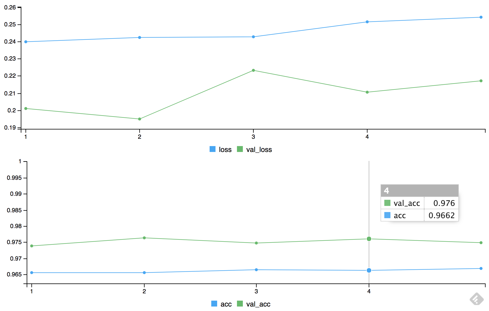
Figure 10.6: Loss functions and accuracy for the training and validation data sets
It is interesting that the plots show the validation sample does better than the training sample. Therefore, there is definitely no overfitting of the model.