Chapter 7 Training Neural Networks Part 1

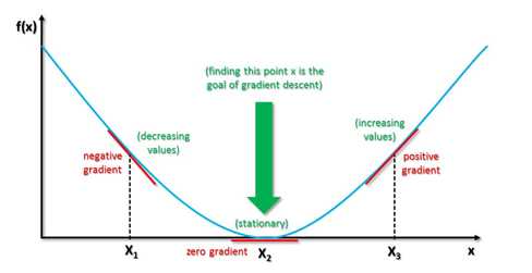
Figure 7.1: Illustrating Gradient Descent

The Backprop algorithm was known by the mid-1980s, but it toook almost two more decades before the field of Deep Learning entered the mainstream. There were several reasons for this delay, including the fact that the processing power was not yet there, but the main reason was that Backprop simply did not work for large models that arise in practical problems. In these cases it was observed that the gradients died away before the training was complete, thus limiting the accuracy of the model. In this chapter and in the next, our objective is go through individual elements of the Gradient Descent algorithm and make improvements so that it is able to work for large models. We start by examining the parameter update equation and present several modifications that improve upon it in Sections 7.2 and 7.3 . We then investigate the role of the Activation Function in Section 7.4, and also come up with a number of alternative functions that improve performance. The correct initialization of weights at the start of the algorithm is also a huge issue, and is discussed in Section 7.5. In Section 7.6 we show that if the training data is pre-conditioned before being fed into the model, then it leads to several benefits in the training process. We end the chapter with a discussion of Batch Normalization which is a recently discovered technique to improve the training process, but which has already had a big impact on the field.

7.1 Issues with Gradient Descent

Recall that the Gradient Descent based parameter update equation in one dimension is given by: \[ w\leftarrow w - \eta\frac{\partial {\mathcal L}}{\partial w} \] As shown in Figure 7.1, \(\frac{\partial {\mathcal L}}{\partial w} > 0\) for points on the curve to the right of the minimum. This causes the value of \(w\) to decrease, until it converges to the minimum point at which the gradient is zero. Conversely \(\frac{\partial {\mathcal L}}{\partial w} < 0\) for points to the left of the minimum, which causes \(w\) to increase with each iteration. There are a number of cases in which this simple iteration does not work very well, and we will describe these next:

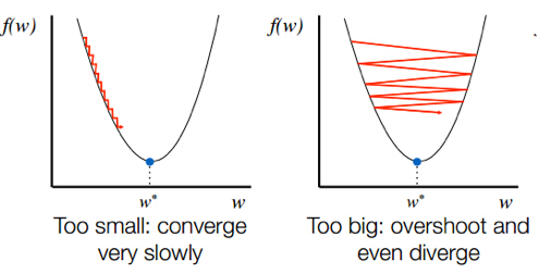
Figure 7.2: Influence of Learning Rate Parameter

1. Even in the simple one dimensional case, it is easy to see that the learning rate parameter \(\eta\) exerts a powerful infuence on the convergence process (see Figure 7.2). If \(\eta\) is too small, then the convergence happens very slowly as shown in the left hand side of the figure. On the other hand if \(\eta\) is too large, then the algorithm starts to oscillate and may even diverge.

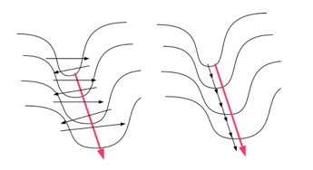
Figure 7.3: Gradient Descent Down a Narrow Steep Valley

2. If Gradient Descent is run in multiple dimensions, then other problems can arise. One such problem is illustrated in Figure 7.3. The figure illustrates a two dimensional scenario in which te Loss Function \(L\) has a very steep slope along one dimension and a shallow slope along the other: i.e., it has the shape of a Narrow Steep Valley. If we run Gradient Descent in this system, we get the behavior shown in the diagram on the LHS (this is a 2-D analog of the behavior shown in the RHS of Figure 7.2). The parameter that lies along the steep part of the objective function oscillates back and forth between the valley slopes, while the parameter that lies along the shallow part of the Loss Function moves slowly down the valley. The net effect of this is that convergence happens very slowly. The right hand side of the figure shows a more ideal convergence behavior, which we will show how to achieve in Section 7.3.

Figure 7.4: Saddle Points

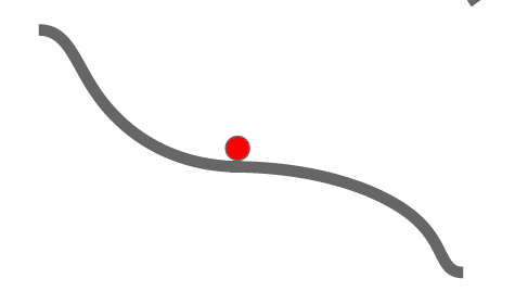
Figure 7.5: Getting Stuck at a Saddle Point

3. Another issue that arises when Gradient Descent is run in multiple dimensions, is that of Saddle Points. These are defined as areas on the surface of the Loss Function, which are a minima when observed along one of the dimensions, and simultaneously serve as a maxima when observes along another dimension. This is illustrated for the the two dimensional case in Figure 7.4. When the iteration approaches a saddle point from above, then even though it is not at a minimum, it slope hits zero. As a result the ieration comes to halt and the algorithm gets stuck a non-optimal point. This bevavior is further illustrated in Figure 7.5.

All the issues with Gradient Descent that were raised in this section are addressed by techniques described in the next two sections.

7.2 Learning Rate Annealing

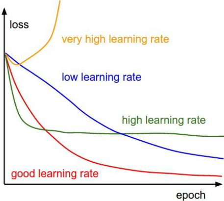
Figure 7.6: Effect of Learning Rate on the Loss Function

As we mentioned in the previous section, the Learning Rate parameter has a big influence on the effectiveness of the Gradient Descent algorithm. If it is set to a large value then the algorithm moves quickly at the start of the iteration, but the large step size can cause a parameter overshoot as the system approaches minimum which can lead to oscillations. If set too small then the algorithm converges with high likelihood, however it can take a very long time to do so (see Fig. 7.2). Hence ideally \(\eta\) should be set adaptively such it is large in the initial stages of the optimization and becomes smaller as it gets closer to the minimum.

Figure 7.6 illustrates the effect of the Learning Rate on the Loss Function during training and can be used to do a quick check on the suitability of the rate being used. A very high Learning Rate can cause the Loss Function to start to increase after a few iterations, while a moderately high rate causes the Loss to plateau at a high value after an initial rapid decrease. A very low Learning Rate on the other hand can be identified by a slow decrease in the Loss Function over training epochs. A good Learning Rate on the other hand combines a quick decrease during the initial epochs with a lower steady state value.

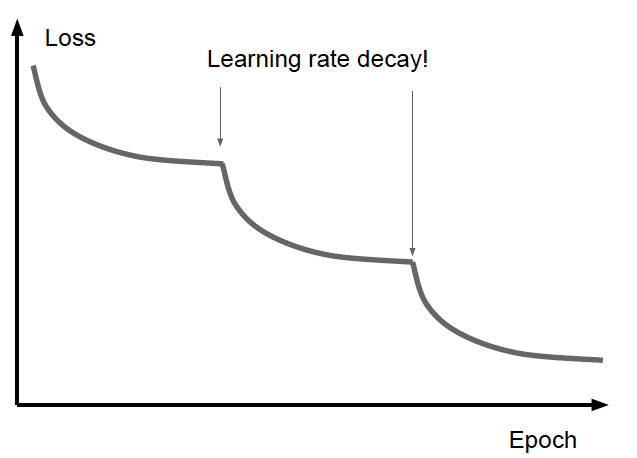
Figure 7.7: Learning Rate Annealing

A well known technique for achieving the best Learning Rate behavior is called Learning Rate Annealing. This is the strategy of reducing the Learning Rate as the system approaches the minimum (see Figure 7.7), such that rate is high at the start of the training and gradually falls as the training progresses. This reduction can be done in several ways, popular approaches are:

• Track the validation accuracy and decrease the Learning Rate when it appears to plateau.

• Automatically anneal the Learning Rate based on the number of epochs that the Gradient Descent algorithm has been through.

Instead of using the same Learning Rate for every parameter, in the next Section we will learn about techniques that tailor the rate to the parameter. Thus parameters possessing a steep gradient get lower rates compared to parameters with a smaller gradient.

7.3 Improvements to the Parameter Update Equation

In the next few sections we present a number of modifications to the base parameter update equation \(w\leftarrow w - \eta\frac{\partial {\mathcal L}}{\partial w}\), which help to improve the performance of the Gradient Descent algorithm. Some of these algorithms automatically adapt the effective Learning Rate as the training progresses (for example the ADAGRAD, RMSPROP and Adam algorithms), while others improve the speed of convergence (for example the Momentum, Nesterov Momentum and Adam algorithms).

7.3.1 Momentum

Momentum is one of the most popular techniques used to improve the speed of convergence of the Gradient Descent algorithm. The basic idea behind Momentum is the following: Some Loss Funtions are characterized by the figure shown on LHS of Figure 7.3. In this case the gradient along one of the dimensions is very large, while along the other dimension it is small. If we do the Gradient Descent iteration for this system then the parameter on the steep side fluctuates from one side of the “canyon” to the other, while the parameter on the shallow side progresses very slowly down the canyon. This behavior slows down the speed of convergence quite a lot. An ingenious but simple technique that can counteract this behavior is as follows: Replace the Gradient Descent iteration by the following:

At the end of the \(n^{th}\) iteration of the Backprop algorithm, define a sequence \(v(n)\) by

\[ v(n) = \rho\; v(n-1) - \eta \; g(n) \] with

\[ v(0) = -\eta \; g(0) \]

where \(\rho\) is new hyper-parameter called the “momentum” parameter, and \(g(n)\) is the gradient evaluated at parameters value \(w(n)\), defined by \[ g(n) = \frac{\partial {\mathcal L(n)}}{\partial w} \] for Stochastic Gradient Descent and \[ g(n) = {\eta\over B}\sum_{m=nB}^{(n+1)B}\frac{\partial {\mathcal L(m)}}{\partial w} \] for Batch Stochastic Gradient Descent (note that in this case \(n\) is an index into the batch number). The change in parameter values on each iteration is now defined as \[\begin{equation} w(n+1) = w(n) + v(n) \tag{7.1} \end{equation}\] It can be shown from these equations that \(v(n)\) can be written as \[\begin{equation} v(n) = - \eta\sum_{i=0}^n \rho^{n-i} g(i) \tag{7.2} \end{equation}\] so that \[\begin{equation} w(n+1) = w(n) - \eta\sum_{i=0}^n \rho^{n-i} g(i) \tag{7.3} \end{equation}\]

When the momentum parameter \(\rho = 0\), then this equation reduces to the usual Stochastic Gradient Descent iteration. On the other hand, when \(\rho > 0\), then we get some interesting behaviors:

• If the gradients \(g(i)\) are such that they change sign frequently (as in the steep side of Figure 7.3), then the stepsize \(\sum_{i=0}^n \rho^{n-i}g(i)\) will be small. Thus the change in these parameters with the number of iterations will limited.

• If the gradients \(g(i)\) are such that they maintain their sign (as in the shallow portion of Figure 7.3), then the stepsize \(\sum_{i=0}^n \rho^{n-i}g(i)\) will be large. This means that if the gradients maintain their sign then the corresponding parameters will take bigger and bigger steps as the algorithm progresses, even though the individual gradients may be small.

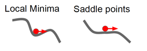
Figure 7.8: Escaping Saddle Points and Local Minima with Momentum

The Momentum algorithm thus accelerates parameter convergence for parameters whose gradients consistently point in the same direction, and slows parameter change for parameters whose gradient changes sign frequently, thus resulting in faster convergence (this is shown on the RHS of Figure 7.3). The variable \(v(n)\) is analogous to velocity in a dynamical system, while the parameter \(1-\rho\) plays the role of the co-efficient of friction. The value of \(\rho\) determines the degree of momentum, with the momentum becoming stronger as \(\rho\) approaches \(1\). Note that \[ \sum_{i=0}^{n} \rho^{n-i}g(i) \le {g_{max}\over 1-\rho} \] \(\rho\) is usually set to the neighborhood of \(0.9\) and from the above equation it follows that \(\sum_{i=0}^n \rho^{n-i}g(i)\approx 10g\) assuming all the \(g(i)\) are approximately equation to \(g\). Hence the effective gradient in Equation (7.3) is ten times the value of the actual gradient. This results in an “overshoot” where the value of the parameter shoots past the minimum point to the other side of the bowl, and then reverses itself. This is a desirable behavior since it prevents the algorithm from getting stuck at a saddle point or a local minima, since the momentum carries it out from these areas (see Figure 7.8).

7.3.2 Nesterov Momentum

Nesterov Momentum is a variation on the plain Momentum method described above. Note that the Momentum parameter update equations can be written as: \[ v(n) = \rho\; v(n-1) - \eta \; g(w(n)) \] \[ w(n+1) = w(n) + v(n) \] In the first equation we have explicitly written out the fact that the gradient \(g\) is computed for parameter value \(w(n)\). These equations can be improved by evaluation of the gradient at parameter value \(w(n+1)\) instead. This may seem like circular reasoning since in order to compute \(w(n+1)\) we first need to compute \(g(w(n))\). However note that \(w(n+1)\approx w(n) + \rho v(n-1)\). This leads to the velocity update equation for Nesterov Momentum \[ v(n) = \rho\; v(n-1) - \eta \; g(w(n)+\rho v(n-1)) \] where \(g(w(n)+\rho v(n-1))\) denotes the gradient computed at parameter values \(w(n) + \rho v(n-1)\). By using a slightly more accurate estimate of the gradient in each step, it has been observed in practice that the Gradient Descent process speeds up considerably when compared to the plain Momentum method.

7.3.3 The ADAGRAD Algorithm

The Momentum and Nesterov Momentum algorithms help to improve the speed of convergence, however we still have the issue of optimally varying the Learning Rate parameter (see Section 7.2). It would be nice if this could be done automatically as part of the parameter update equation and this is precisely what the ADAGRAD algorithm does. This algorithm replaces the parameter update rule with the following equation:

\[\begin{equation} w(n+1) = w(n) - \frac{\eta}{\sqrt{\sum_{i=1}^n g(n)^2+\epsilon}}\; g(n) \tag{7.4} \end{equation}\]

The constant \(\epsilon\) has been added to better condition the denominator and is usually set to a small number such \(10^{-7}\). Equation (7.4) leads to the following benefits: Each parameter gets its own adaptive Learning Rate, such that large gradients have smaller learning rates and small gradients have larger learning rates (\(\eta\) is usually defaulted to \(0.01\)). As a result the progress along each dimension evens out over time, which helps the training process. This is a type of Learning Rate annealing, but it is more powerful since:

• Each parameter gets its own customized rate,
• The change in rates happens automatically as part of the parameter update equation.

Also, the accumulation of gradients in the denominator leads to smaller Learning Rates over time, which has the same effect as annealing. This is a double edged sword, since the continuous decrease in Learning Rates can lead to a halt of training in large networks that require a greater number of iterations. This problem is addressed by the RMSPROP algorithm, which is described next.

7.3.4 The RMSPROP Algorithm

The RMSPROP algorithm accumulates the sum of gradients using a sliding window, using the following formula: \[ E[g^2]_n = \rho E[g^2]_{n-1} + (1-\rho) g(n)^2 \] where \(\rho\) is a decay constant (usually set to \(0.9\)). This operation (called a Low Pass Filter) has a windowing effect, since it forgets gradients that are far back in time. The quantity \(RMS[g]_n\) defined by \[ RMS[g]_n = \sqrt{E[g^2]_n + \epsilon} \] is used in the denominator of equation (7.4), resulting in following the parameter update equation: \[\begin{equation} w(n+1) = w(n) - \frac{\eta}{RMS[g]_n}\; g(n) \tag{7.5} \end{equation}\]

Note that \[ E[g^2]_n = (1-\rho)\sum_{i=0}^n \rho^{n-i} g(i)^2 \le \frac{g_{max}}{1-\rho} \] which shows that the parameter \(\rho\) prevents the sum from blowing up, and a large value of \(\rho\) is equivalent to using a larger window of previous gradients in computing the sum. Hence RMSPROP retains the benefits of ADAGRAD while avoiding the decay of the Learning Rate to zero.

7.3.5 The Adam Algorithm

The Adaptive Moment Estimation (Adam) algorithm combines the best of algorithms such as Momentum that speed up the training process, with algorithms such as RMSPROP that adaptively vary the effective Learning Rate. The update equtions for Adam are as follows:

\[ \Lambda(n) = \beta\Lambda(n-1) +(1-\beta)g(n),\ \ \ {\hat\Gamma}(n) = \frac{\Gamma(n)}{1-\beta^n} \] \[ \Delta(n) = \alpha\Delta(n-1) + (1-\alpha) g(n)^2,\ \ \ {\hat\Delta}(n) = \frac{\Delta(n)}{1-\alpha^n} \] \[ w(n+1) = w(n) - \eta\frac{\hat\Lambda(n)}{\sqrt{\hat\Delta(n) + \epsilon}} \] The definition of the sequence \(\Delta(n)\) is identical to that of \(E[g^2]_n\) in the RMSPROP, and it serves an identical purpose, i.e., it is used to customize the effective Learning Rate on a per parameter basis, so that the rates for parameters with larger gradients are equalized with those for parameters with smaller gradients.

The sequence \(\Lambda(n)\) is used to provide “Momentum” to the updates, and works in a fashion similar to the velocity sequence \(v(n)\) in the Momentum algorithm. It is easy to show that \[ \Lambda(n) = (1-\rho)\sum_{i=0}^n \rho^{n-i} g(i) \le \frac{g_{max}}{1-\rho} \] which shows that \(\Lambda(n)\) is the weighted sum of the previous \(n\) gradients (compare this with the expression for \(v(n)\) in Equation (7.2)). Since \(\Lambda(n)\) and \(\Delta(n)\) are initialized as vectors of 0’s, they are biased towards 0 at the start of the iteration. These biases are counteracted by computing the estimates \(\hat\Lambda(n)\) and \(\hat\Delta(n)\). The parameters \(\alpha\) and \(\beta\) are usually defaulted to \(10^{-8}\) and \(0.999\) respectively.

Adam serves as the default choice for the parameter update rule, since it combines the best features of the other update algorithms.

7.4 Choice of Activation Functions

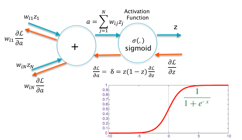
Figure 7.9: Problem with Sigmoids

The choice of Activation Function has a major influence on the training and operation of DLN systems. When DLNs were first proposed, the first choice for the activation was the sigmoid, probably as a result of what was then known about biological neurons. This turned out to be an unfortunate choice, as illustrated in Figure 7.9. This picture shows a single neuron with a sigmoid activation. Using the Gradient Flow rules from Chapter 6, we can see that the backpropagation of the gradient \(\frac{\partial\mathcal L}{\partial z}\) results in \[\frac{\partial\mathcal L}{\partial a} = z(1-z)\frac{\partial\mathcal L}{\partial z}\] If the neuron is saturated, i.e., \(a\) lies significantly away from the origin, then from the shape of the sigmoid it follows that either \(z\) or \((1-z)\) is zero, which implies that \(\frac{\partial\mathcal L}{\partial a} \approx 0\). As a result the gradients flowing back to the next layer of nodes will also be zero. The neuron in this state is said to be “dead”. Once a neuron is dead, it stays dead, since in order to get get it back into the active state, the inputs weights (shown on the LHS of Figure 7.9) need to change. However the weights cannot change since the gradient with respect to the weights is given by \(\frac{\partial\mathcal L}{\partial w} = z'\delta\) and \(\delta = 0\).

Thus the choice of the sigmoid function contributed to the Vanishing Gradient problem that plagued the first DLN systems. Interestingly enough, a suitable replacement for the sigmoid (the ReLU function) was not proposed until 2010. But once it was in place, it contributed to the rapid advances in the field since then. Our objective in this section is to survey some of the many Activation Functions that have been proposed in the last few years.

7.4.1 The tanh Function

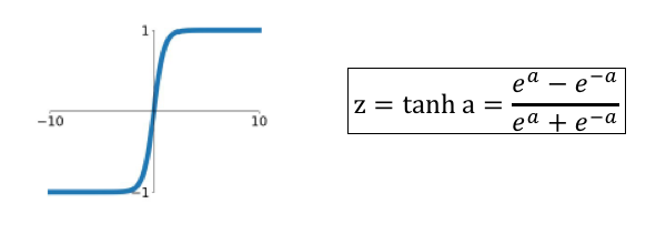
Figure 7.10: The tanh Activation Function

Historically the \(\tanh\) function was proposed next after the sigmoid. As Figure 7.10 shows, its shape is very similar to the sigmoid, so that unless the input is in the neghborhood of zero, the function enters its saturated regime. It is superior to the sigmoid in one respect, i.e., its output is zero centered. This is a desirable property in Activation Functions, since we show later in Section @ref(#DataPreprocessing), that this speeds up the training process. The \(\tanh\) function is rarely used in modern DLNs, the exception being a type DLN called LSTM (see Chapter 13). Some of the variables in LSTMs function as memory units, in which \(\tanh\) outputs are used to increment or decrement the memory state by numbers that are close to \(+1\) or \(-1\).

7.4.2 The ReLU Function

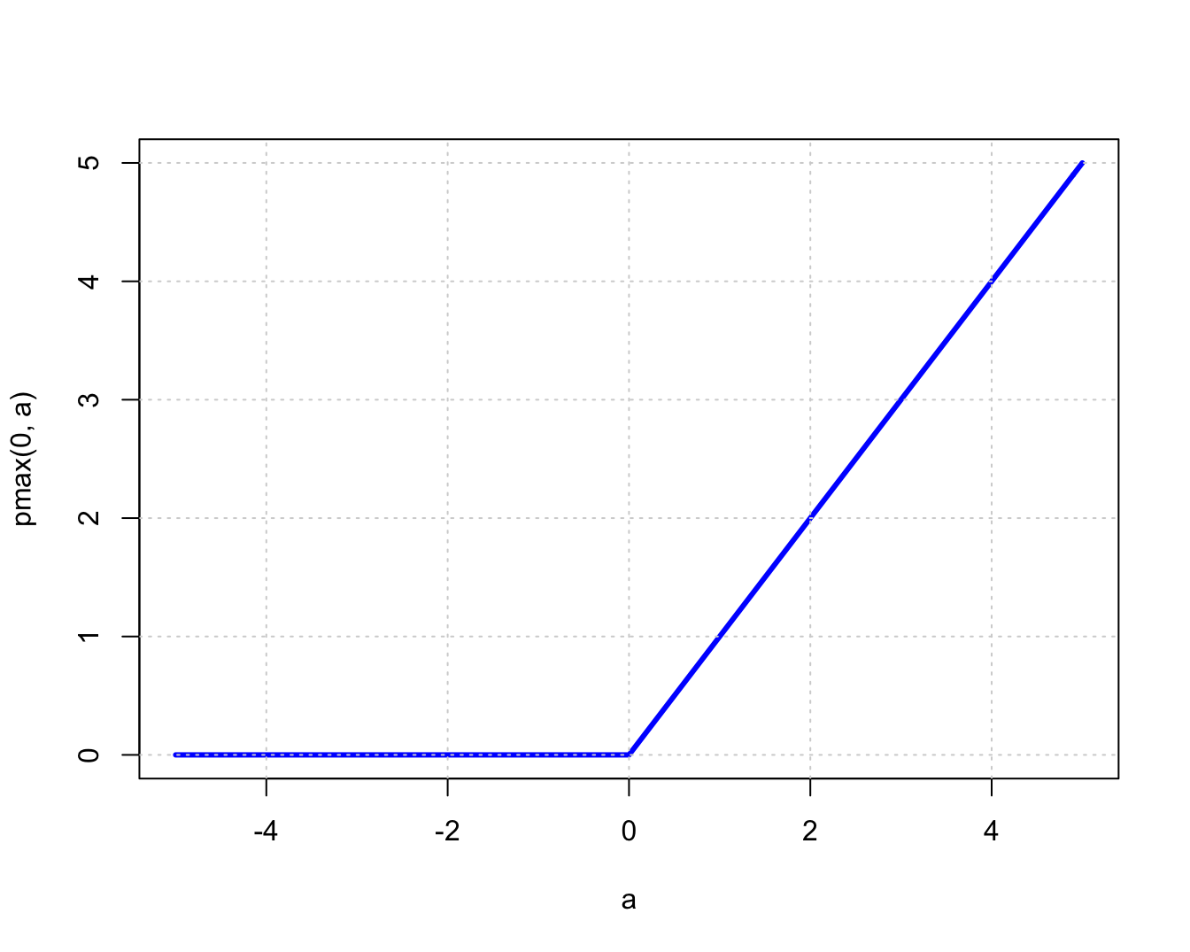
Figure 7.11: The Rectified Linear Unit (ReLU) Activation Function

The most common Activation Function in use today is the Rectified Linear Unit or ReLU (see 7.11). This function was proposed in 2010 by Nair and Hinton (2010) as a replacement for the sigmoid. The function is given by:

\[ z = \max(0,a) \]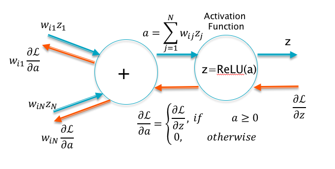

Figure 7.12: ReLU as a Switch

This is an extremely simple Activation Function which is linear with slope one for positive values of the argument, and zero otherwise. Hence this function does not suffer from the saturation problem as long as the input exceeds zero. Furthermore since the slope is one for \(x>0\) and zero for \(x<0\), it follows that it functions as a gate controlled by its input during the backprop process (see Figure 7.12). It follows that the gradients \(\frac{\partial L}{\partial w}\) propagate undiminished through the network, provided all the nodes are active. This makes DLNs using ReLU less susceptible to Vanishing Gradients.

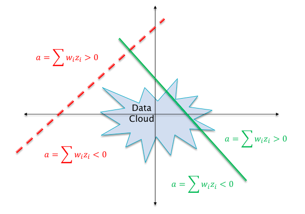
Figure 7.13: The Dead ReLU Problem

Even though ReLU based DLNs are much better at propagating gradients compared to what came before, they do suffer suffer from the “Dead ReLU Problem”. This is illustrated in Figure 7.13. The dotted line in this figure shows a case in which the weight parameters \(w_i\) are such that the hyperplane \(\sum w_i z_i\) does not intersect the “data cloud” of possible input activations. This implies that there does not exist any possible input values that can lead to \(\sum w_i z_i > 0\). Hence the neuron’s output activation will always be zero, and it will kill all gradients backpropagating down from higher layers. This is referred to as the “Dead ReLU” problem. When training large networks with millions of neurons, it is not un-common to run into a situation in which a section of the network becomes dead and takes no further part in the training process. In order to avoid this, the DLN designer should be on the alert to spot this situation and take steps to correct it. The problem is most often caused due to bad initializations and later in this chapter we will show how to properly initialize a network to avoid this. The hyperplane for a well functioning neuron is shown as the solid line in Figure 7.13. Note that it intersects with the input data cloud so that there are input values that put the neuron in the active state.

Over the last few years, several other Activation Functions have been proposed, but none of them offer a significant performance benefit over the ReLU function, which remains the most widely used. A couple of popular functions are described next.

7.4.3 The Leaky ReLU and the PreLU Functions

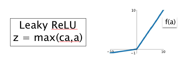
Figure 7.14: The Leaky ReLU Function

The Leaky ReLU function is shown in Figure 7.14 and is defined by: \[ z = \max(ca,a),\ \ 0\le c<1 \] where \(c\) is a hyper-parameter representing the slope of the function for \(a<0\). The idea behind this function is quite straighforward, it backpropagates a gradient of \(c\) if the input \(a<0\), thus avoiding the Dead ReLU problem.

Instead of deciding on the value of \(c\) through experimentation, why not determine it using Backpropagation as well. This is the idea behind the Pre-ReLU or PReLU function shown in Figure 7.15.

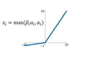
Figure 7.15: The PreLU Function

This function is defined as

\[ z_i = \max(\beta_i a_i,a_i), \quad 1 \le i \le S \] Note that each neuron \(i\) now has its own parameter \(\beta_i, 1\le i\le S\), where \(S\) is the number of nodes in the network. These parameters are iteratively estimated using Backprop. In order to do this we use the Gradient Flow rules to obtain an expression for the gradient \(\frac{\partial\mathcal L}{\partial\beta_i}\) as follows: \[ \frac{\partial\mathcal L}{\partial\beta_i} = \frac{\partial\mathcal L}{\partial z_i}\frac{\partial z_i}{\partial\beta_i},\ \ 1\le i\le S \] Substituting the value for \(\frac{\partial z_i}{\partial\beta_i}\) we obtain \[ \frac{\partial\mathcal L}{\partial\beta_i} = a_i\frac{\partial\mathcal L}{\partial z_i}\ \ if\ a_i \le 0\ \ \mbox{and} \ \ 0 \ \ \mbox{otherwise} \] which is then used to update \(\beta_i\) using \(\beta_i\rightarrow\beta_i - \eta\frac{\partial\mathcal L}{\partial\beta_i}\). Once training is complete, the PreLU based DLN network ends up with a different value of \(\beta_i\) at each neuron, which increases the flexibility of the network at the cost of an increase in the number of parameters.

7.4.4 The MaxOut Function

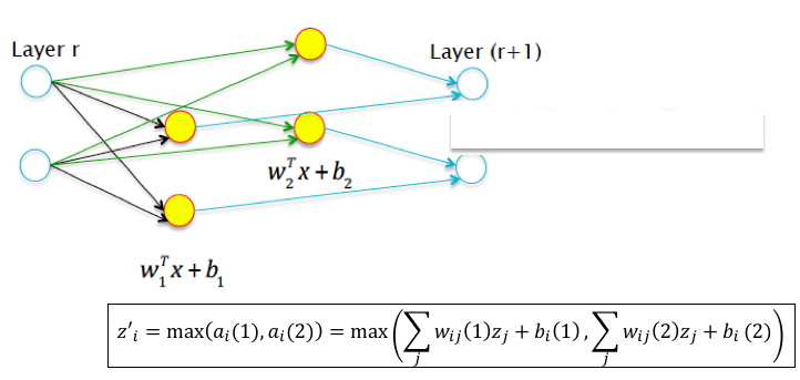
Figure 7.16: Maxout for the case k = 2

In order to motivate the design of the Maxout function, consider the Leaky ReLU function: \[ z = \max(ca,a), \] This can also be written as (using \(z_i\) for the input activations and \(z'_i\) for the output activations): \[ z'_i = \max(c\big[\sum_j w_{ij}z_j +b_i\big],\sum_j w_{ij}z_j +b_i), \] Hence the output activation is the max of two hyperplanes, one of which is a multiple of the other. A straightforward generalization of this is shown in Figure 7.16, in which we allow the two hyperplanes to be independent with their own set of parameters, i.e., \[ z'_i = \max(\sum_j w_{ij}(1)z_j +b_i(1),\sum_j w_{ij}(2)z_j +b_i(2)) \] and we have arrived at the Maxout function.

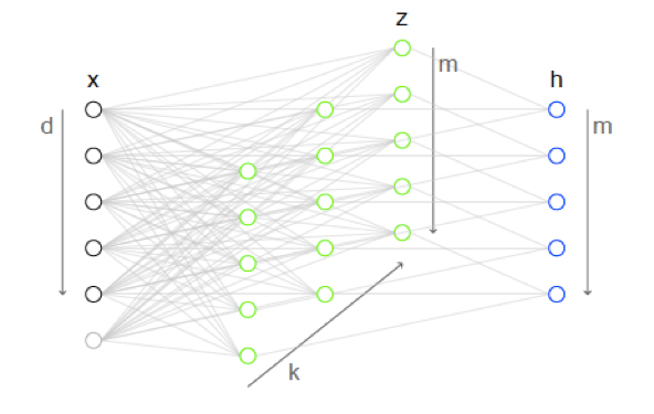
Figure 7.17: Illustration of the Maxout Activation Function

As shown in Figure 7.17 , this idea can be generalized so that each activation is the max of \(k\) hyperplanes. In the absence of Maxout, the layer on the left with \(d\) nodes (marked \(x\)) would be fully connected to the later on the right with \(m\) nodes (marked \(h\)). Maxout introduces \(k\) additional layers in-between, each of them with \(m\) nodes. The nodes in these “hidden layers” compute an affine function \(a_{ij}\) (at the \(i\)-th node of the \(k\)-th hidden layer), without a corresponding Activation:

\[ a_{ij} = z^\top W_{\_ij} + b_{ij}, \quad 1 \leq i \leq m, 1 \leq j \leq k \]

Note that \(W\) is now a Tensor of dimension \(d \times m \times k\), while \(b\) is now a matrix of dimension \(m \times k\).

The final output at the \(i\)-th output node, which is the Activation Function that we are after, is then computed as the maximum of the outputs of the \(k\) nodes at the \(i\)-th position in the “hidden layers”.

\[ z'_i = \max_{1 \leq j \leq k} a_{ij}, \quad 1 \leq i \leq m \]

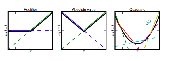
Figure 7.18: Function Synthesis using Maxout

Figure 7.18 shows examples of Activation Functions that have been synthesized out of linear segments by following the Maxout algorithm. Hence a single maxout node can be interpreted as making linear approximation to an arbitrary convex activation function, whose shape is learnt as part of the training process. The Maxout function works quite well in practice, but at the expense of a large increase in the number of parameters.

7.5 Initializing the Weight Parameters

The choice of the initialization for DLN weight parameters is an extremely important decision, and can determine whether the Stochastic Gradient algorithm converges successfully or not. A bad initialization can lead to a premature end of the training process with all the activations and gradients going towards zero, or numerical instabilities and failure to converge. Even when the algorithm does converge successfully, the initial point can determine the speed of convergence, the end value of the Loss Function, the classification accuracy on the test set, etc.

Unfortunately, due to lack of theoretical understanding of the DLN optimization process, we rely on a few simple heuristics for doing initialization that have been discovered over the years. One of the only rules in this area which is known with certainty is that the initial parameters should be set in such a way as to “break symmetry” between nodes. This means that if two nodes have the same set of inputs, then they need to be initialized to different values, or else the stochastic gradient iteration being deterministic, will cause their values to change in lock step.

In practice, the DLN weight parameters are initialized with random values drawn from Gaussian or Uniform distributions and the following rules are used:

• Guassian Initialization: If the weight is between layers with \(n_{in}\) input neurons and \(n_{out}\) output neurons, then they are initialized using a Gaussian random distribution with mean zero and standard deviation \(\sqrt{2\over n_{in}+n_{out}}\).

• Uniform Initialization: In the same configuration as above, the weights should be initialized using an Uniform distribution between \(-r\) and \(r\), where \(r = \sqrt{6\over n_{in}+n_{out}}\).

When using the ReLu or its variants, these rules have to be modified slightly (see He et al. (2015b)):

• Guassian Initialization: If the weight is between layers with \(n_{in}\) input neurons and \(n_{out}\) output neurons, then they are initialized using a Gaussian random distribution with mean zero and standard deviation \(\sqrt{4\over n_{in}+n_{out}}\).

• Uniform Initialization: In the same configuration as above, the weights should be initialized using an Uniform distribution between \(-r\) and \(r\), where \(r = \sqrt{12\over n_{in}+n_{out}}\).

The reasoning behind scaling down the initialization values as the number of incident weights increases is to prevent saturation of the node activations during the forward pass of the Backprop algorithm, as well as large values of the gradients during backward pass.

7.6 Data Preprocessing

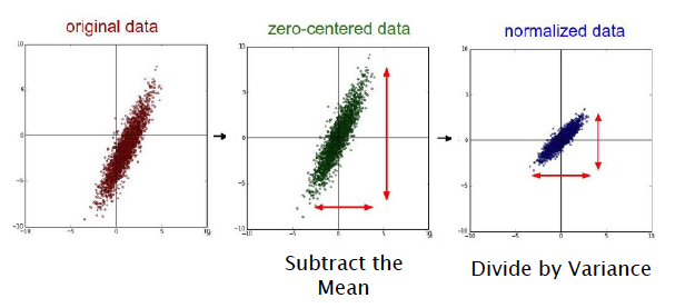
Figure 7.19: Data Pre-Processing

Data Preprocessing is an important step in all ML systems, including DLNs. Data Preprocessing steps include cleaning, normalization, transformation, feature extraction and selection etc. Kotsiantis and al. (2006) is a well known reference on this topic, and has descriptions of these steps. In this section we describe only the Normalization step, which is the process of Data Centering + Scaling. Normalization is applied most commonly in DLN systems used to process image data. These operations are illustrated in Figure 7.19.

Data Normalization and proceeds in the following steps:

• Centering: This is also sometimes called Mean Subtraction, and is the most common form of preprocessing. Given an input dataset consisting of \(M\) vectors \(X(m) = (x_1(m),...,x_N(m)), m = 1,...,M\), it consists of subtracting the mean across each individual input component \(x_i, 1\leq i\leq N\) such that \[ x_i(m) \leftarrow x_i(m) - \frac{\sum_{s=1}^{M}x_i(s)}{M},\ \ 1\leq i\leq N, 1\le m\le M \] This has the geometric interpretation of centering the data around the origin for each dimension as shown in the center illustration in Figure 7.19. A color image consists of three channels of RGB pixels \((X^R(m),X^G(m),X^B(m)\))$. The following two techniques have been used to center images of this type:
  • Subtract the Mean Image: For CH = R, G, B, \[ x^{CH}_{ij}(m) \leftarrow x^{CH}_{ij}(m) - \frac{\sum_{s=1}^{M}x_{ij}^{CH}(s)}{M},\ \ 1\leq i,j\leq N, 1\le m\le M \] This equation assumes that each image consists three channels of NxN pixels. The mean value of each pixel is computed across the entire training set. This results in a “Mean Image” of size NxNx3 which is then subtracted from the individual pixel values.
  • Subtract the Per-Channel Mean: \[ x^{CH}_{ij}(m) \leftarrow x^{CH}_{ij}(m) - \frac{\sum_{s=1}^M\sum_{i=1}^N\sum_{k=1}^N x_{ij}^{CH}(s)}{M},\ \ 1\leq i,j\leq N, 1\le m\le M \] This is a simpler normalization technique in which a single mean value is computed for each channel, and then subtracted from the data in that channel.
• Scaling: After the data has been centered, it can be scaled in one of two ways:
  • By dividing by the standard deviation, once again along each dimension, so that the overall transform is \[ x_i(m) \leftarrow \frac{x_i(m) - - \frac{\sum_{s=1}^{M}x_i(s)}{M}}{\sigma_i},\ \ 1\leq i\leq N, 1\le m\le M \]
  • By Normalizing each dimension so that the min and max along each axis are -1 and +1 repectively. In general Scaling helps optimization because it balances out the rate at which the weights connected to the input nodes learn. For image processing applications Scaling shows limited benefits, hence image pre-processing is limited to Centering.

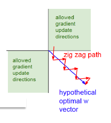
Figure 7.20: Why Zero Centering Helps

We end this section by giving an intuitive explanation of why the Centering operation helps to speed up convergence. Recall that for a K-ary Linear Classifier, the parameter update equation is given by: \[ w_{kj} \leftarrow w_{kj} - \eta x_j(y_k-t_k),\ \ 1\le k\le K,\ \ 1\le j\le N \] If the training sample is such that \(t_q = 1\) and \(t_k = 0, j\ne q\), then the update becomes: \[ w_{qj} \leftarrow w_{qj} - \eta x_j(y_q-1) \] and \[ w_{kj} \leftarrow w_{kj} - \eta x_j(y_k),\ \ k\ne q \] Lets assume that the input data is not centered so that \(x_j\ge 0, j=1,...,N\). Since \(0\le y_k\le 1\) it follows that \(\Delta w_{kj} = -\eta x_jy_k <0, k\ne q\) and \(\Delta w_{qj} = -\eta x_j(y_q - 1) > 0\), i.e. the update results in all the weights moving in the same direction, except for one. This is shown graphically in Figure 7.20, in which the system is trying move in the direction of the blue arrow which is the quickest path to the minimum. However if the input data is not centered, then it is forced to move in a zig-zag fashion as shown in the red-curve.The zig-zag motion is caused due to the fact that all the parameters move in the same direction at each step due to the lact of zero-centering in the input data.

7.7 Batch Normalization

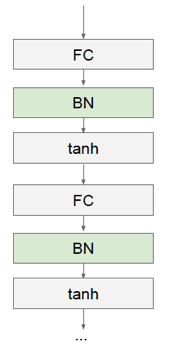
Figure 7.21: Batch Normalization

Data Normalization at the input layer was described in the previous section as a way of transforming the data in order to speed up the optimization process. Since Normalization is so beneficial, why not extend it to the interior of the network and normalize all activations. This is precisely what is done in an algorithm called Batch Normalization (Ioffe and Szegedy (2015)). This technique has led to a signficant improvement in the performance of DLN models, indeed the ResNet model that won the 2015 ILSVRC competition made extensive use of Batch Normalization (He et al. (2015a)).

It was a straightforward exercise to apply the Normalization operations to the input data, since the entire training data set is available at the start of the training process. This is not case with the hidden layer activations, since these values change over the course of the training due to the algorithm driven updates of system parameters. Ioffe and Szegady solved this problem by doing the normalization in batches (hence the name), such that during each batch the parameters remain fixed.

Batch Normalization proceeds as follows: As shown in Figure 7.21, we introduce a new layer between the Fully Connected and the Activation layers. This layer is responsible for doing centering and scaling for the pre-activation sums \(a_i^{(k)}\), before it is passed through the non-linearity.

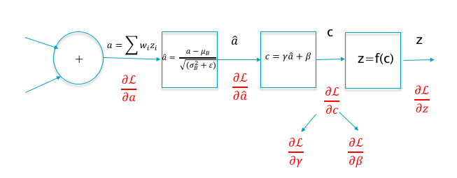
Figure 7.22: Backprop for Batch Normalization

1. Let \(a(m),1\leq m\leq B\) denote the \(m^{th}\) pre-activation value in a training batch of size B, where we have omitted the subscripts \(i\) and \(k\) for clarity. Then the algorithm computes the following values (see Figure 7.22): \[ \mu_B = \frac{1}{B}\sum_{m=1}^{B}a(m) \] \[ \sigma_B^2 = \frac{1}{B}\sum_{m=1}^B (a(m)-\mu_B)^2 \] \[ \hat{a}(m) = \frac{a(m)-\mu_B}{\sqrt{\sigma_B^2+\epsilon}} \] \[c(m) = \gamma\hat{a}(m) + \beta \] This is done on a Layer-by Layer basis so that the normalized outputs of layer \(r\) are fed into layer \(r+1\), which is then normalized.

2. Run Backprop for each of the samples in the batch using the normalized activations. In addition to the weights, compute the gradients for the parameters \((\gamma,\beta)\) at each node.

3. Average the gradients across the batch and use them to update the weight and batch normalization parameters.

4. Go back to step 1 and repeat for the next batch

5. During the test phase, once the network has been trained, the pre-activations are normalized using the mean and variance for the entire training set, rather than just the batch.

The algorithm introduces new parameters \(\gamma\) and \(\beta\) whose values are estimated using the backprop iteration. Note that at each layer, the algorithm processes all B vectors in the batch in parallel, so that the resulting pre-activation \(c(m)\) is influenced not just by its own input \(x(m)\), but also by the other inputs in the batch. This is the same as introducing noise into the system, since we are letting each classification decision be influenced by more than one piece of input data. In the next chapter we will see that this functions as a kind of Regularizer which improves the generalization performance of the system on the Test dataset.

Much of the power of the Batch Normalization technique arises from the following: We first normalize the pre-activations so that they have zero mean and unit variance, but then in the very next step we re-introduce a mean and variance through the parameters \((\gamma,\beta)\). But note that these re-introduced values are actually learnt as part of the Gradient Descent algorithm, so they assume values that are more suited to the task of minimizing the loss function.

Batch Normalization has been shown to lead to several benefits, including:

• It enables higher learning rates: In a non-normalized network, a large learning rate can lead to oscillations and cause the loss function increase rather than decrease. Batch Normalization helps prevents these problems by preventing small changes in the parameters from amplifying into larger and sub-optimal changes in activations and gradients. Higher learning rates in turn speed up the training process considerably.

• It enables better Gradient Propagation through the network, thus enabling DLNs with more hidden layers.

• It helps to reduce strong dependencies on the parameter initialization values.

• It helps to regularize the model. Regularization is a process that we discuss in the next chapter and has to do with the ability of the model to generalize beyond its training set. Indeed experiments show that Batch Normalization reduces the need to use other regularization techniques such as Dropout (see Chapter 8).

7.8 The Vanishing Gradient Problem

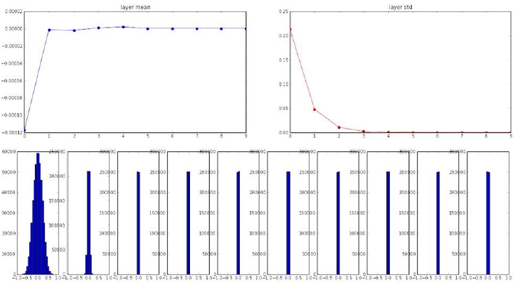
Figure 7.23: Distribution of Activation Values - 1

We mentioned at the start of this chapter that there was a twenty year gap between the time the Backprop algorithm was discovered, and when DLNs entered the mainstream. Most of this delay can be attributed to a problem called Vanishing Gradients. The issues that caused this problem were gradually recognized and addressed by the techniques and algorithms described in this chapter.

The main reason for the prevalance of Vanishing Gradients in early DLNs was a combination of bad initializations and the use of sigmoid functions for activations. The importance of proper parameter initializations was not appreciated in the early DLNs, as a result they were frequently initialized using a Normal distribution with mean 0 and small variance, such as \(N(0,0.01)\). Figure 7.23 plots the mean, variance and the distributions for the activations at each of the layers in the DLN. The first layer shows a healthy distribution, however we progress deeper into the network, the variance rapidly falls to zero as does the mean. This is mainly due to the fact that the weights are very small, and successive layers keep multiplying them over and over again. Since the gradient with respect to the weights is given by the product of the activations and \(\delta\) (= \(\frac{\partial L}{\partial a}\)) \[ \frac{\partial L}{\partial w} = z\delta \] it follows that the gradients will also go to zero. If we were to initialize the weights using a large variance such as \(N(0,1)\), this did not solve the problem either, since it causes the sigmoid activation to go into saturation, this killing the gradients \(\delta\) (as explained in Section 7.4) and causing \(\frac{\partial L}{\partial w}\) to once again go to zero.

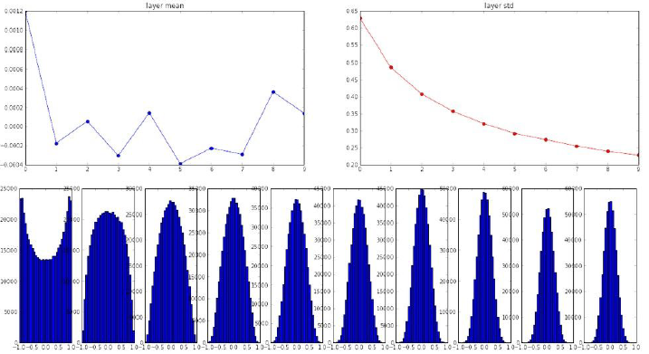
Figure 7.24: Distribution of Activation Values - 2

The discovery of the initialization rules described in Section 7.5 combined with replacement of sigmoids by ReLU (as well as Data Preprocessing describes in Section 7.6) all helped to put the Vanishing Gradient Problem to rest. Figure 7.24 shows the graphs for the activation function statistics in a well functioning DLN which incorporates all these techniques, and it canbe seen that the activation distributions even in the deeper layers have a good spread, which shows that the network is continuing to learn from new training data.

References

Nair, Vinod, and Geoffrey Hinton. 2010. “Rectified Linear Units Improve Restricted Boltzmann Machines.” ICML.

He, Kaiming, Xiangyu Zhang, Shaoqing Ren, and Jian Sun. 2015b. “Delving Deep into Rectifiers: Surpassing Human-Level Performance on Imagenet Classification.” CoRR abs/1502.01852. http://arxiv.org/abs/1502.01852.

Kotsiantis, S. B., and et al. 2006. “Data Preprocessing for Supervised Learning.”

Ioffe, Sergey, and Christian Szegedy. 2015. “Batch Normalization: Accelerating Deep Network Training by Reducing Internal Covariate Shift.” CoRR abs/1502.03167. http://arxiv.org/abs/1502.03167.

He, Kaiming, Xiangyu Zhang, Shaoqing Ren, and Jian Sun. 2015a. “Deep Residual Learning for Image Recognition.” CoRR abs/1512.03385. http://arxiv.org/abs/1512.03385.