Chapter 2 Pattern Recognition
Pattern Recognition is the task of classifying an image into one of several different categories. Since their inception, Pattern Recognition is the most common problem that NNs have been used for, and over the years the increase in classification accuracy has served as an indicator of the state of the art in NN design. The MNIST pattern recognition problem served as a benchmark for DLN systems until recently, and in this section we introduce DLNs by describing the problem and the way in which they are used to solve it.
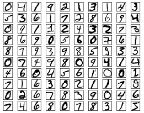
Figure 2.1: A Portion of the the MNIST Handwritten Digits database
The MNIST database consists of 70,000 scanned images of handwritten digits from 0 to 9, a few of which are shown in Figure 2.1. Each image has been digitized into a \(28 \times 28\) grid, with each of the 784 pixels in the grid assigned a quantized grayscale value between 0 and 1, with 0 representing white and 1 representing black. These numbers are then fed into a DLN as shown in Figure 2.2. We will go into the details of the DLN architecture in Chapter 5, but at a high level the reader can observe that the DLN shown in Figure 2.2 has three layers of nodes (or neurons). The layer on the left is the Input Layer and consists of 784 neurons, with each neuron assigned a number with the grayscale value of the corresponding pixel from the input image. Note that the 2-dimensional image has been stretched out into a 1-demensional vector before being fed into the DLN. The middle layer is called the Hidden Layer and consists of 15 neurons, while the third layer is called the Output Layer and consists of 10 neurons. As the name implies, the Output Layer indicates the output of the DLN computation, so that ideally if the input corresponds to the digit \(k\), \(0 \leq k \leq 9\) , then the \(k^{th}\) output neuron should be 1, and the other 9 should be zero.
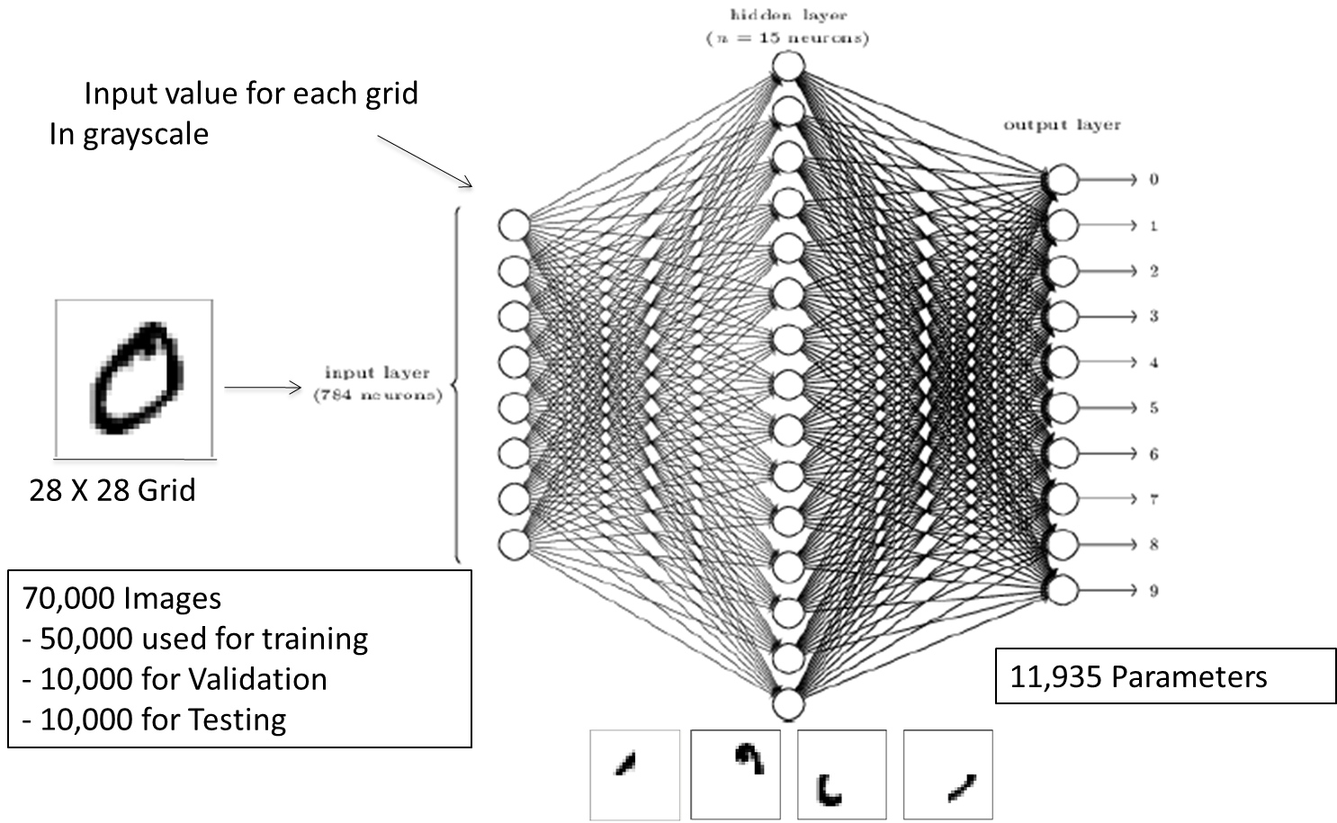
Figure 2.2: The NN used for Solving the MNIST Digit Recognition Problem
The neurons in the Input and Hidden Layers are fully connected which implies that each neuron in the input layer is connected to every neuron in the Hidden Layer (and the same goes for the neurons between the Hidden and Output Layers). Note that these connections are uni-directional, i.e. exist in the forward direction only. Each of these connections is assigned a weight and each node in the Hidden and Output layers is assigned a bias, so that there are a total of \(784 \times 15 + 15 \times 10 +15 +10 = 11,935\) weight + bias parameters needed to describe the network.
In an operational network, these 11,935 weight and bias parameters have to be set, so that the DLN is able to do its job. The process of choosing these parameters is known as “training the network” and uses a learning algorithm that proceeds by iteration. After the training is complete, the DLN should be able to classify images of digits that were not part of the training dataset, which is known as the networks “Generalization Ability”.
The system operates as follows:
The 70,000 images in the MNIST database are divided into 3 groups: 50,000 images are used for training the DLN (called the training dataset), 10,000 images are used for choosing the model’s hyper-parameters (called the validation dataset) and the remaining 10,000 images are used for testing (called the test dataset).
The training process operates as follows:
The grayscale values for an image in the training data set are fed into the Input Layer. The signals generated by this propagate through the network, called forward propagation, and the values at the Output Layer are compared with the desired output (for example if the image is of the digit 2, then the desired output should be 0100000000). A measure of the difference between the desired and actual values is then fed back into the network and propagates back, using an algorithm known as Backprop. The information gleaned from this process is then used to modify all the link weights and node bias values, so that the desired and actual outputs are closer in the next iteration.
The process described above is repeated for each of the 50,000 images in the training set, which is known as a training Epoch. The network may be trained for multiple epochs until a stopping condition is satisfied, usually the error rate on the Validation data set should fall below some threshold.
Other than the weights and biases, there are some other important model parameters that are part of the training process, known as hyper-parameters. Some of these hyper-parameters are used to improve the optimization algorithm during training, while others are used to improve the model’s generalization ability. The training data is also used to find the best values for these hyper-parameters while using the validation data set for verification testing.
- After the network is fully trained, the 10,000 images in the test dataset are used to test the DLN’s classification accuracy.
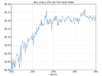
Figure 2.3: Accuracy as a function of the number of Epochs
Figure 2.3 plots the accuracy of the classification process as a function of the number of Epochs using the test data set. As can be seen, the classification accuracy increases almost linearly initially, but after about 260 Epochs, the classification accuracy does not increase beyond 82.25% or so (in other words the NN classifies about 8225 images correctly out of a total of 10,000 Test Images). The reasons why the testing accuracy plateaus out and what can be done to increase it further forms the subject of Section 8. In practice, the best accuracy that has been achieved by a state of the art NN on the MNIST classification problem is about 99.67%, i.e., only 33 mis-classifications out of 10,000!
Figure 2.2 also provides some insight into how the DLN is able to carry out the classification task, for the example in which the input is a handwritten zero. In a trained NN, four of the nodes in the Hidden layer are tuned to recognize the presence of dark pixels in certain parts of the image, as shown in the bottom of the figure. This is done by appropriately choosing the weights on the links between the Input and Hidden layers, which is also called filtering. As shown in the figure, the output node that corresponds to the digit 0, filters these 4 Hidden layer nodes (by setting the weights on the links between the Hidden and Output layers), such that its own output tends towards 1, while the outputs of the other nodes in the Output layer tend towards 0.
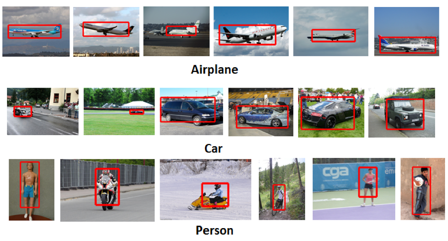
Figure 2.4: Some Images from the ILSVRC data set
While the MNIST data set played an important role in the early years of Deep Learning, current systems have become powerful enough to be able to handle much more complex image classification tests. ImageNet is an on-line data set consisting of 16 million full color images obtained by crawling the web. These images have been labeled using Amazon’s Mechanical Turk service, and some example are given in Figure 2.4. A popular Machine Learning competition called ImageNet Large-Scale Visual Recognition Challenge (ILSVRC) uses a 1.2 million subset of these images, drawn from 1,000 different categories, with 50,000 images used for validation and 150,000 for testing. In recent years the ILSVRC competition has served as a benchmark for the best DLN models. For example the 2014 competition was won by a network called the GoogLeNet with 22 layers of nodes, which achieved an accuracy of 93.33%.