Chapter 13 Recurrent Neural Networks

13.1 Introduction

Recurrent Neural Nets or RNNs, are DLN systems that are designed to detect patterns present in sequences. This makes them well suited to solve “prediction” problems, as opposed to regular DLNs that are oriented to solving classification problems. An example of a prediction problem is predicting the next word in a sentence, which is a problem that occurs in language translation or captioning tasks. The solution to this problem requires that the system take into account the words that came before, i.e., it should be able to “remember” previous data in the sequence. Just like ConvNets, RNNs were discovered in the late 1980s, but lay dormant until recently due to the difficulty in training them. These problems have been overcome in recent years, with the use of a type of RNN called Long Short Term Memory or LSTMs, as well as the increase in processing power and size of training datasets. Today RNNs are at the forefront of exciting new discoveries in Deep Learning, and some of the most important recent work in DLNs falls in the RNN domain.

In order to motivate the need for RNNs, consider the following: The DLN architectures that we have seen so far implement a static mapping between input and ouput vectors, of the type \[ Y=f(X) \] Instead, consider a system that is evolving with time, i.e., it is a Dynamical System. In this scenario, the system is subject to an input sequence \(X_1,...,X_n\) and results in an output sequence \(Y_1,...,Y_n\). Furthermore the output vector \(Y_i\) at time \(i\) depends not just on the input vector \(X_i\), but on past values of \(X\) as well, i.e., \[ Y_i = f_i(X_1,...,X_i) \] Systems with this type of dependency are commonly encountered in practice and are usually studied by postulating a Hidden Variable or Hidden State \(Z_i\) (also called a State Variable) The evolution of the system state obeys the following recursion: \[ Z_{i+1} = w_{i+1}(Z_i,X_i) \] while the output is a function of the current state and is given by \[ Y_{i+1} = v_{i+1}(Z_{i+1}) \] The Hidden Variable sequence \(Z_i\) captures the lossy history of the \(X_i\) sequence, and hence serves as a type of memory. If we assume that the functions \(v\) and \(w\) do not change with time, then these equations reduce to:

\[ \begin{equation} Z_{i+1} = w(Z_i,X_i) \tag{13.1} \end{equation} \]

\[ \begin{equation} Y_{i+1} = v(Z_{i+1}) \tag{13.2} \end{equation} \]

Traditional Systems Theory makes the additional simplifying assumption that these functions are linear so that \[ Z_{i+1} = WZ_i + UX_i \]

\[ Y_{i+1} = VZ_{i+1} \] The use of DLNs enables us to approximate non-linear functions to high degree of accuracy using the training dataset, so that this linearity assumption is no longer needed. We do however assume that the vectors \(Z_i\) and \(X_i\) can be combined linearly, so that the resulting equations are:

\[ \begin{equation} Z_{i+1} = f(W Z_i + UX_i) \tag{13.3} \end{equation} \]

\[ \begin{equation} Y_{i+1} = h(V Z_{i+1}) \tag{13.4} \end{equation} \]

Equations (13.3) and (13.4) are in a form in which they can be implemented using Neural Networks, with the functions \(f\) and \(h\) serving as the Activation Functions, as shown in Figure 13.1.

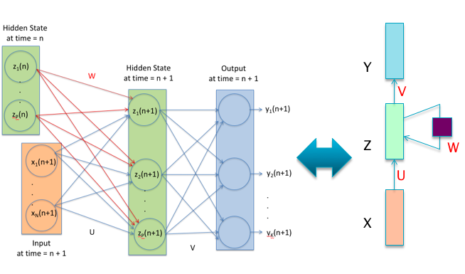
Figure 13.1: A Recurrent Neural Network

The figure shows three types of nodes:

\(X{(n)}\): This represents the value of the input vector at time \(n\).

\(Z{(n)}\): This represents the value of the Hidden Layer vector at time \(n\).

\(Y{(n)}\): This represents the value of the output vector at time \(n\).

The LHS of Figure 13.1 shows a RNN with connections between the Hidden Layers at times \(n\) and \(n+1\) shown explicitly. The RHS of Figure 13.1 is a simplified representation of the same RNN. Each of the boxes in this figure represents a row of Neural Network nodes belonging to a single layer, of the type shown on the LHS, which have been omitted for the sake of clarity. Note that:

• The weight matrix \(U\) connects the nodes in the Input Layer with those in the Hidden Layer
• The weight matrix \(W\) connects the nodes in the Hidden Layer with the same set of nodes, but at the previous time instant. The square block on the self-loop to the Hidden Layer represents a time delay of one unit, and represents the fact that at time \(n\), the nodes in that layer have as one of their inputs, the values that they had at time \(n-1\)
• The weight matrix \(V\) connects the nodes in the Hidden Layer with those in the Output Layer.

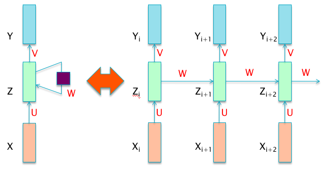
Figure 13.2: An Unfolded Recurrent Neural Network

The fact that all these weight matrices do not change with time is a result of the time invariance assumption. While Figure 13.1 accurately captures the fact that the RNN design incorporates feedback, it does not lend itself easily to training of the type we have seen in deep feed-forward DLNs. In order to facilitate the reuse of techniques we have developed in previous chapters, we convert Figure 13.1 into an equivalent feed-forward DLN network shown in Figure 13.2, by a process called “unfolding”. The RHS of Figure 13.2 basically shows snapshots of the DLN at various points in time, and the fact that there is feedback between the nodes in the Hidden Layer is captured by the connections involving the weight matrix \(W\). As a result of the unfolding operation, the system becomes amenable to optimization using the Backprop algorithm. In addition, the depth of the RNN is now dependent on the length of the input data sequence. This can result in a RNN with hundreds of Hidden Layers, hence the problems of training deep models with Backprop have a special resonance here. We also mentioned earlier that the Hidden Layer in RNNs keeps a “Lossy Memory” of the input sequence - the reason why it is lossy is because this single layer has to capture data from an entire input sequence, which cannot be done without compressing the data is some fashion.

In order to gain an intuitive understanding of the way in which the RNN shown in Figure 13.2 operates, note the following: There is an analogy between the way a ConvNet operates by looking for patterns in localized patches of an image, and the way a RNN operates by looking for patterns in localized intervals in time. Just as a ConvNet slides a single Filter over the entire image, a RNN slides its own filter represented by the weight matrix U over the entire input sequence, one input at a time. Hence RNNs implement a form of Translational Invariance, but they do this over the temporal axis, as opposed to spatial Translational Invariance seen in ConvNets. As a result of this property, the important part of the sequence can occur anywhere along the time axis, but still can be detected using a single weight matrix repeated at each point in time. There is however a crucial difference in the way a RNN operates compared to a ConvNet: Due to the feedback loop, the RNN pattern detector in the Hidden Layer is able to take advantage of the information that was learnt in the prior time steps from older data in the sequence. As a result the RNN is able to detect patterns that are spread over time, something that a ConvNet cannot do (in the spatial sense).

There is a fundamental difference between the internal representations that are created in the hidden layers of a ConvNet vs those that are created in the hidden layers of a RNN. The hidden layers in a ConvNet create a hierarchical representation, in which the representation at layer \(r+1\) is at a higher level of abstraction compared to that for layer \(r\). The hidden layer in a RNN on the other hand, does not add to the level of abstraction in the representation with successive time steps. Instead it captures patterns that are spread in time, but at the same level of abstraction. It is indeed possible to combine DLNs and RNNs and create deep RNNs (see the next section for examples), in which case higher level hidden layers capture time dependent patterns at different levels of abstraction.

The rest of this chapter is organized as follows: RNNs can be configured in several useful ways depending upon the problem they are being used to solve, some of these are described in Section 13.2. In Section 13.3 we discuss the training of RNNs and the problems that arise when doing so. In particular the Backprop algorithm can lead to issues such as the Vanishing Gradients Problem or the Exploding Gradient Problem, and in Section 13.4 we discuss a modified RNN architecture called LSTM (Long Short Term Memory) which was designed to solve these problems. Section 13.6 is on applications of RNNs to problems such as Machin Translation, Speech Transcription and Image Captioning. As part of this we introduce the concept of Langauge Modeling using RNNs in Section @ref(RNN_LMs). We end the chapter in Section 13.7 with a discussion of some recent development in incorporating memory into DLNs using a RNN like structure.

13.2 Examples of RNN Architectures

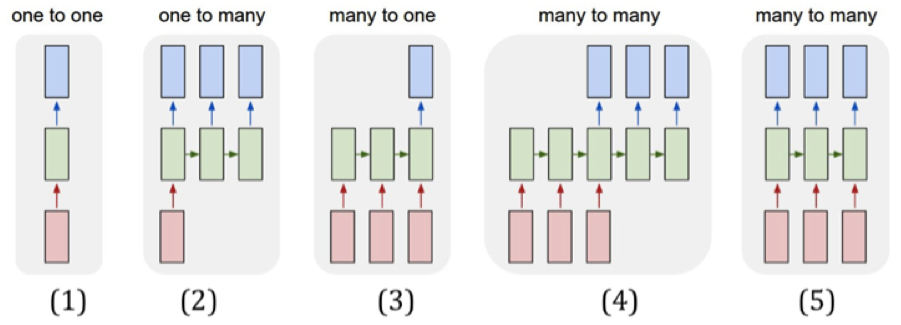
Figure 13.3: RNN Architectures

RNNs can be configured in a number of useful ways depending upon the problem they are being used to solve, which is one of their big architectural strengths. Some of these configurations are shown in Figures 13.3 and 13.4. Continuing the convention used in Figure 13.1, we use a single box to represent an entire layer of nodes.

• In these diagrams the (red) input box can be one of the following: (a) A scalar value: For example simple RNN models of stock indices fall in this category, (b) A vector: Examples include embedded representations for words or samples from a sound waveform, (c) 2-D structures: For example black and white images, (d) 3-D structures: For example color images.
• The (green) Hidden Layer can be one of the following: (a) A simple 1-D layer or multiple 1-D layers of neurons, as those found in deep feed forward networks, or more complicated structures (see Figure 13.4), (c) 2-D structures in one or more layers, such as convolutional layers in ConvNets. In this case the system would correspond to a hybrid of RNNs and ConvNets.
• The (blue) Output Layer in most cases consists of a single layer of Logit neurons, which are used to compute the classification probabilities.

We describe these architectures in more detail next:

• Part (1) of the Figure 13.3 shows a vanilla DLN for comparison purposes, in which a single input is mapped to an output.

• Part (2) of the figure shows a RNN architecture that is used to map a single input, to a variable number of outputs. As we will see later in this chapter, this design can be used to generate image captions. In this application, the input corresponds to an image, information about which is captured by the final layer of a ConvNet and then fed into this RNN. Each output in the RNN maps to a single word of the resulting image caption.

• Part (3) of the figure shows a RNN architecture in which a variable number of inputs are mapped to a single output. Examples of applications of this architecture include a system for mapping a piece of text to a sentiment, i.e., Sentiment Analysis. It can also be used to do video classification, in which case each input is a video frame, and the output is the category to which the video belongs.

• Part (4) of the figure shows an important RNN architecture called Encoder-Decoder. This design is used to map a variable number inputs to a variable number of outputs. Some of the most exciting recent applications of RNNs utilize Encoder-Decoder systems, and are described in Section 13.6. When used for doing Machine Translation, the inputs represent the words of the sentence in Language 1, while the outputs represent the translation in Language 2. When used for Speech Transcription, the inputs represent the sound waveform, while the outputs represent the corresponding words. Encoder-Decoder systems have been much improved lately with the addition of an algorithm called the Attention Mechanism, and they have achieved state of the art performance in all areas that they have been applied to.

• Part (5) of the figure shown a RNN architecture that maps a variable number of inputs is mapped to the same number of outputs, such that there is a one-to-one mapping between input-output pairs. This design can be used to do video image classification on a frame-by-frame basis, such that each input corresponds to an image and the corresponding output is the class to which the image belongs.

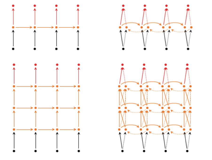
Figure 13.4: Deep RNN Architectures

Figure 13.4 shows some additional ways in which RNN nodes can be configured by borrowing ideas from Deep Feed Forward Networks:

• The figure on the top left is a re-drawing of Part (5) of Figure 13.3, where the boxes have been replaced by the small circles in order to simplify the diagram.

• The figure in the bottom left shows a RNN with multiple hidden layers, usually referred to as a Deep RNN. This system incorporates ideas from Deep Feed Forward Networks into the RNN, and enables the system to simultaneously create: (1) Higher level hierarchical representations of the input data, and (2) At each level of the hierarchy capture temporal patterns in the data. This architecture is used quite commonly in current RNN systems.

• The figure in the top right shows an important RNN architecture called Bi-Directional RNNS. As the name implies this system incorporates two sets of hidden layers. The first set is the conventional hidden layer, with connections going from left to right, while the second set of Hidden Layers has connections going in the opposite direction, from right to left. The output at each time step incorporates information from both the forward and backward hidden layers. Such a design can be used for the case when the input sequence is not being generated in real time. As a result of this architecture, the output is able to take advantage of input patterns from the past, as well as from the future. This can be very beneficial and has been shown to substantially improve performance in many cases.

• The figure in the bottom right is a mashup of the Bi-Directional RNN and the Deep RNN, and incorporates multiples layers of bi-directional hidden nodes.

13.3 Training RNNs: The Back Propagation Through Time (BPTT) Algorithm

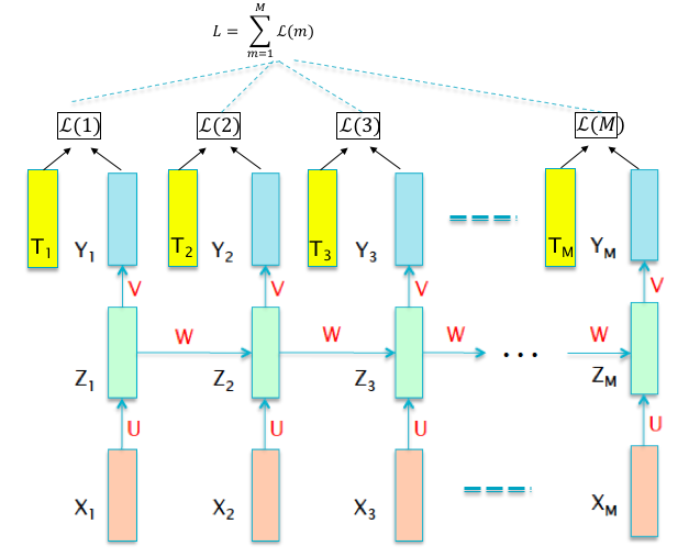
Figure 13.5: Training RNNs

The Backprop algorithm that was described in Chapter 6 can be modified in order to train RNNs, and this forms the subject of this section. We start by setting up the optimization problem, which as before, is to minimize the Loss Function \(L\) (see Figure 13.5). Recall that \(L\) is a function of of the labeled Training Sequence \(\{(X(i),T(i))\}_{i=1}^{M}\) and the network parameters \((W,b)\), so that the it can be written as:

\[\begin{equation} L = \sum_{m=1}^M \mathcal L(m) \tag{13.5} \end{equation}\]

where \(\mathcal L(m)\) is the Cross Entropy Loss Function for the \(m^{th}\) training pair, given by \[ \mathcal L(m) = -\sum_{k=1}^{K}t_k(m)\log y_k(m) \] In this equation \(K\) is the number of output categories, \(t_k(m), 1\le k\le K\) is the Ground Truth vector at the \(m^{th}\) stage, and \(y_k(m), 1\le k\le K\) are the classification probabilities for the \(m^{th}\) stage, given by \[ y_k(m) = \frac{\exp(a_k(m))}{\sum_{j=1}^K \exp(a_j(m))},\ \ 1\le k\le K \] where \(a_k(m), 1\le k\le K\) are the corresponding logits. The overall Loss function can then be written as \[ L=\sum_{m=1}^M \mathcal L(m)= - \sum_{m=1}^M\sum_{k=1}^K t_k(m)\log y_k(m) \] The modification to the Backprop algorithm to train RNNs is called Back Propagation Through Time (BPTT), and we now provide a high level description of this algorithm (detailed calculations are in the following sub-sections):

• Forward Pass: BPTT proceeds in an iterative fashion to compute the activations, as follows:
  • Time Step 1: The computation of \((Y(1), \mathcal L(1))\) in response to the training input \((X(1), T(1))\) proceeds by the usual rules of Deep Feed Forward Networks.
  • Time Step 2: In order to compute \((Y(2), \mathcal L(2))\), both the new training input \((X(2), T(2))\) as well as the Hidden Layer state \(Z(1)\) from the previous time step, are used.
  • Time Steps m = \(3\) to \(M\): These proceed in a similar fashion to time step 2, using both the current training input \((X(m), T(m))\) as well the previous Hidden State \(Z(m-1)\) to compute \((Y(m), \mathcal L(m))\), until \((Y(M), \mathcal L(M)\) is computed at the last step.
• Backward Pass: Once again BPTT uses an iterative procedure, but this is now run backward starting from time step \(M\) and ending at time step \(1\). The logit layer gradients at each time step \(\delta_k^Y(m) = \frac{\partial\mathcal L(m)}{\partial a^Y_k(m)}\) are computed easily using the training data as follows: \[ \delta_k^Y(m) = y_k(m) - t_k(m), 1\le k\le K, 1\le m\le M \] The backward iterations proceed as follows:
  • Time Step \(M\): Applying the usual Backprop rules, use \(\delta_k^Y(M), 1\le k\le K\) to compute the gradients \(\delta_i^Z(M) = \frac{\partial\mathcal L(M)}{\partial z_i(M)}, 1\le i\le P\) at the \(M^{th}\) Hidden Layer.
  • Time Step \(M-1\): Once again use the Backprop rules to compute \(\delta_i^Z(M-1), 1\le i\le P\) by using the gradients \(\delta_k^Y(M-1), 1\le k\le K\) from the current time step, and the hidden layer gradients \(\delta_i^Z(M), 1\le i\le P\) from the next time step.
  • Time Steps \(m = M-2\) to \(1\): These proceed in a similar fashion to time step \(M-1\), using the current logit layer gradients \(\delta_k^Y(m), 1\le k\le K\) as well as the hidden layer gradients \(\delta_i^Z(m+1), 1\le i\le P\) from the next time step.
• Using the node level gradients \(\delta_k^Y(m), \delta_i^Z(m), 1\le k\le K, 1\le i\le P, 1\le m\le M\) to compute the gradients with respect to all the weight parameters \(\frac{\partial\mathcal L}{\partial u_{ij}}, \frac{\partial\mathcal L}{\partial v_{ij}}, \frac{\partial\mathcal L}{\partial w_{ij}}\).
• Use the Stochastic Gradient Descent iteration to update the weight parameters.

13.3.1 Truncated Back Propagation through Time

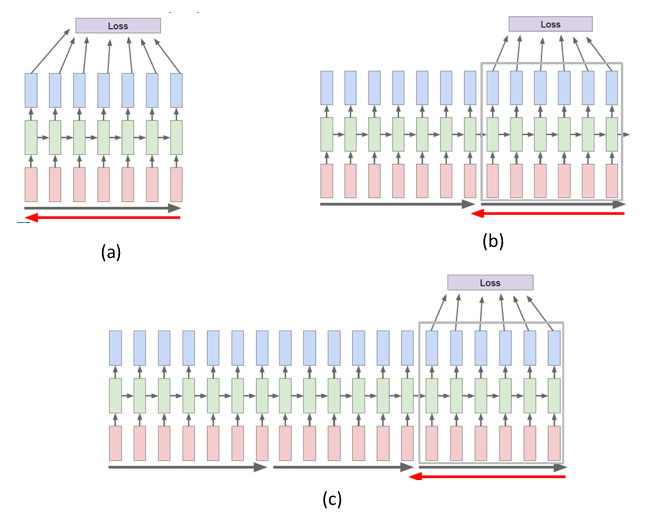
Figure 13.6: Truncated BPTT

Given the structure of RNNs, it is possible to process the entire training sequence \((X(m),T(m)),m=1,..,M\) using a large RNN with M stages. However this is not a good idea, since typically the RNN is not able to keep track of historical data in the past values of the input sequence, beyond 20 or 30 stages. These issue is treated in greater detail in later in this chapter, but for now we describe a training technique that is commonly used to mitigate this problem called Truncated BPTT. This technique is illustrated in Figure 13.6 and the basic idea is to break up the input training sequence into smaller segments, and then run BPTT on each segment at a time. Part (a) of the figure shows BPTT being applied to the first segment, while parts (b) and (c) BPTT being aplied to the second and third segments respectively. However in order to create a connection between successive segments, the final Hidden State vector \(Z\) from segment \(n\) is used as the initial value for the Hidden State vector in segment \(n+1\). It has been observed experimentally that this technique is effective in detecting correlations between inputs that are located more than a segment-size apart.

In the following two sub-sections we give detailed calculations for the forward and backward passes of the BPTT algorithm.

13.3.2 BPTT Forward Pass

The forward pass of the RNN backprop algorithm proceeds as follows (refer to Figure 13.5):

• Step 1: The input vector \(X(1) = (x_1(1),...,x_N(1))\) is applied to the system, resulting in the hidden state activation vector \(Z(1)=(z_1(1),...,z_P(1))\) and the output vector \(Y(1) = (y_1(1),...,y_K(1))\), as per the formulae:

\[ a_i^Z(1) = \sum_{j=1}^{N} u_{ij}x_j(1) + b_i^Z,\quad 1\le i\le P \]

\[ z_i(1) = f(a_i^Z(1)), \quad 1\le i\le P \] and the logits \[ a_k^Y(1) = \sum_{j=1}^{P} v_{kj}h_j(1) + b_k^Y,\quad 1\le k\le K \] \[ y_k(1) = \frac{a_k^Y(1)}{\sum_j a_j^Y(1)},\quad 1\le k\le K \] The Loss Function \(\mathcal L(1)\) is computed using the output vector \(Y(1)\) and the target vector \(T(1)\).

• Step 2: The input vector \(X(2)\) and the hidden state vector \(Z(1)\) is applied to the system, resulting in the hidden state activation vector \(Z(2)\), the output vector \(Y(2)\) and the loss \(\mathcal L(2)\).

\[ a_i^Z(2) = \sum_{j=1}^{N} u_{ij}x_j(2) + \sum_{j=1}^{P}w_{ij}z_j(1) + b_i^Z, \quad 1\le i\le P \] \[ z_i(2) = f(a_i^Z(2)),\quad 1\le i\le P \]

\[ a_k^Y(2) = \sum_{j=1}^{P} v_{kj}z_j(2) + b_k^Y, \quad 1\le k\le K \] \[ y_k(2) = \frac{a_k^Y(2)}{\sum_j a_j^Y(2)},\ \ 1\le k\le K \] Step 2 is repeated an additional \(M-2\) times to compute the vectors \(Z(j), 3\le j\le M\) and \(Y(j), 3\le j\le M\) until the remaining input vectors \((X(3),...,X(M))\) have been processed. This constitutes the forward pass of the BPTT algorithm.

13.3.3 BPTT Backward Pass

Define the following gradients:

\[ \Delta^Y(m) = (\delta_1^Y(m),...,\delta_K^Y(m)),\quad 1\le m\le M \] where

\[ \delta_k^Y(m)= \frac{\partial L}{\partial a_k^Y(m)},\quad 1\le k\le K \] and \[ \Delta^Z(m) = (\delta_1^Z(m),...,\delta_P^Z(m)),\quad 1\le m\le M \] where

\[ \delta_i^Z(m)= \frac{\partial L}{\partial a_i^Z(m)},\quad 1\le i\le P \]

The backward pass proceeds in the following steps:

• Compute the logit gradients \(\Delta^Y(m), 1\le m\le M\) using the formula \[ \delta_k^Y(m)= y_k(m) - t_k(m),\quad 1\le k\le K,\quad 1\le m\le M \] In order to derive this equation, recall that \(L = \sum_{m=1}^M \mathcal L(m)\), so that \[ \frac{\partial L}{\partial a_k^Y(m)} = \sum_{j=1}^M \frac{\partial L}{\partial \mathcal L(j)}\frac{\partial \mathcal L(j)}{\partial a_k^Y(m)} = \frac{\partial L}{\partial \mathcal L(m)}\frac{\partial \mathcal L(m)}{\partial a_k^Y(m)} = \frac{\partial \mathcal L(m)}{\partial a_k^Y(m)} = y_k(m) - t_k(m) \] We used the fact the \(\frac{\partial \mathcal L(j)}{\partial a_k^Y(m)} = 0\) except when \(j = m\) when deriving the above equation.

• Similarly it is possible to show that \[ \frac{\partial L}{\partial a_i^Z(m)} = \frac{\partial \mathcal L(m)}{\partial a_i^Z(m)},\quad 1\le i\le P,\ 1\le m\le M \] which results in the following formula for the components of the vector \(\Delta^Z(M)\): \[ \delta_i^Z(M) = f'(a_i^Z(M))\sum_{j=1}^{K}v_{ji}\delta_j^Y(M),\quad 1\le i\le P \]

• Use the following equation to compute the components of the vectors \(\Delta^Z(m), m = M-1, M-2,...,1\) recursively: \[ \delta_i^Z(m)=f'(a_i^Z(m))[\sum_{j=1}^{K}v_{ji}\delta_j^Y(m) + \sum_{j=1}^P w_{ji}\delta_j^Z(m+1)]\quad 1\le i\le P,\quad m=M-1,M-2,...,1 \]

• The gradient of the Loss Function with respect to the weight matrices \(U, V, W\) is then given by the sum of the gradients across each of the stages, as shown below:

\[ \frac{\partial L}{\partial u_{ij}} = \sum_{m=1}^M x_j(m)\delta_i^Z(m)\quad 1\le j\le N,\quad 1\le i\le P \]

\[ \frac{\partial L}{\partial v_{kj}} = \sum_{m=1}^M z_j(m)\delta_k^Y(m)\quad 1\le j\le P,\quad 1\le k\le K \]

\[ \frac{\partial L}{\partial w_{ij}} = \sum_{m=1}^{M-1} z_j(m)\delta_i^Z(m+1)\quad 1\le j\le P,\quad 1\le i\le P \]

The justification for the summation is identical to the argument presented in Section 12.5 in the context of shared filter weights in ConvNets. For example, consider the weight \(u_{ij}\) which connects the \(j^{th}\) node in each of the Input Layers with the \(i^{th}\) node in each of the Hidden Layers. This implies that the Loss Function \(L\) is influenced by \(u_{ij}\) through each of the pre-activations \(a_i^Z(m), 1\le m\le M\), so that

\[ \frac{\partial L}{\partial u_{ij}} = \sum_{m=1}^M \frac{\partial L}{\partial a^Z_{i}(m)}\frac{\partial a_i^Z(m)}{\partial u_{ij}} = \sum_{m=1}^M x_j(m)\delta_i^Z(m) \]

A similar set of equations can be derived for the gradients of the Loss Function with respect to the bias parameters, and is left to the reader.

13.3.4 Difficulties with Backprop in RNNs

When the BPTT algorithm, is applied to a RNN with a large number of stages, then we run into some problems that were first encountered when training Fully Connected DLNs, but they have more serious implications for RNNs:

• The Vanishing Gradient Problem: As a result of the Vanishing Gradient Problem, the gradients \(\delta^Z_i\) become progressively smaller and get close to zero as the number of RNN stages increases.

• The Exploding Gradient Problem: This leads to the opposite effect, i.e., the gradients \(\delta^Z_i\) become larger and larger as we add more RNN stages.

The causes of these problems can be understood by analysing the recursion equations for the gradients, and we proceed to do this next. The gist of the argument can be understood by considering a simple scalar sequence \(\{x_n\}\) generated by the recursion: \[ x_{n+1} = ax_{n} \ \ {\mbox so}\ \ that\ \ x_{n} = a^n x_0,\ \ n=1,2,... \] Clearly if \(a<1\) then the sequence converges to zero, while if \(a>1\), then the sequence blows up to infinity. In the case of RNNs, the BPTT recursion equations for the gradients \(\delta^Z_i = \frac{\partial L}{\partial a^Z_i}\) are given by (after ignoring the contribution from the logit gradients \(\delta^Y_k\)) \[ \delta^Z_i(m) = f'(a_i^Z(m))\sum_{j=1}^P w_{ji}\delta^Z_j(m+1),\ \ 1\le i\le P,\ \ m = M-1, M-2,...,1 \] Using matrix notation, this recursion can be written as \[ \Delta^Z(m) = f'(A^Z(m))\odot W^T\Delta^Z(m+1) \] where \(W^T\) is the transpose of the weight matrix \(W\). Ignoring the derivative \(f'\) (and noting that since with ReLUs, \(f'\) is either \(1\) or \(0\), this is a reasonable assumption), it follows that \[ \Delta^Z(M-n) = (W^T)^n\ \Delta^Z(M),\ \ n = 1,2,...,M-1 \] If the matrix \(W\) can be decomposed as \[ W = R\Lambda R^T \] where \(R\) is an orthogonal matrix, and \(\Lambda\) is a diagonal matrix with the eigenvalues \(\lambda_i\) at the \(i^{th}\) position along the diagonal. The (backwards) recursion then becomes \[ \Delta^Z(M-n) = R^T\Lambda^n R\ \ \Delta^Z(M),\ \ n = 1, 2,...,M-1 \] Note that the diagonal matrix \(\Lambda^n\) has components \(\lambda^n\), and as \(n\) increases, they either converge to \(0\) if \(\lambda < 1\) (resulting in Vanishing Gradients) or go to infinity if \(\lambda > 1\) (resulting in Exploding Gradients). Hence for larger values of \(M\), this will result in the gradients \(\delta^Z_i\) of the early stages converging to zero.

In the previous section we derived the following expression for the gradient of the Loss Function with respect to the weight parameters \(W\): \[ \frac{\partial L}{\partial w_{ij}} = \sum_{m=1}^{M-1} z_j(m)\delta_i^Z(m+1),\quad 1\le j\le P,\quad 1\le i\le P \] Combining this equation with the prior one, it follows that the node activations \(z_j(m)\) from the early stages of the network will have limited or no effect on the gradient \(\frac{\partial L}{\partial w_{ij}}\). This is known as the problem of Long Term Dependencies in RNNs, i.e., in a RNN with a large number of stages, the early training samples are not able to influence the gradients, and thus the learning process.

13.3.5 Solutions to the Vanishing and Exploding Gradients Problems

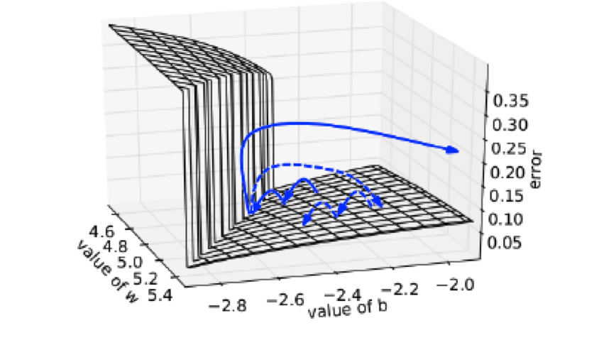
Figure 13.7: Illustration of Gradient Clipping

The Exploding Gradient problem is usually addressed by a technique known as Gradient Clipping. As the name implies, this involves clipping the gradients \(\frac{\partial L}{\partial w}\) whenever they explode,i.e., if their value exceeds some pre-set threshold, then it is set back to a small number. Defining \[ {\hat g}=\frac{\partial L}{\partial W} \] If \(||{\hat g}|| \ge threshold\) then \[ {\hat g} \leftarrow \frac{threshold}{||{\hat g}||}{\hat g} \] The effect of Gradient Clipping is illustrated in Figure 13.7, in which the Loss Function is plotted as a function of the network parameters \((w,b)\). The solid blue arrows show the progression of the Loss Function with successive optimization steps. When the optimization hits the high Loss Function wall, then the next gradient will be extremely large, and in the absence of Gradient Clipping, the Loss Function is pushed off to a distant location on the Loss Function surface. On the other hand, with Gradient Clipping the optimization proceeds along the dashed line, where we can see that the Loss Function is pulled back to an area that is closer to its original location.

The Vanishing Gradient problem can be (partially) addressed by using Truncated BPTT which restricts the number of stages over which BPTT is run to twenty or less. This technique doesn’t work well in all cases and in general the Vanishing Gradient problem is more difficult to solve using traditional RNNs. In the next section we describe an alternative RNN architecture which was designed with the objective of solving this problem.

13.4 Long Short Term Memories (LSTMs)

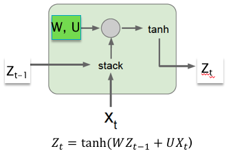
Figure 13.8: A RNN Cell

LSTMs were designed with the objective of solving the Vanishing Gradients Problem that plagues RNNs. They have been very successful in this regard, indeed almost all of the successful applications of RNNs in recent years have been with LSTMs rather than with plain RNNs.

In order to understand LSTM design, we start with Figure 13.8 which illustrates a single stage of a typical RNN, which we call a Cell. Each Cell uses two weight parameter matrices \(W\) and \(U\). Using the tanh Activation Function, it operates on the Hidden Layer vector \(Z_{t-1}\) from the previous stage and the input \(X_t\) from the current stage, and uses the following equation to generate a new Hidden Layer vector \(Z_t\): \[ Z_t = \tanh(WZ_{t-1} + UX_t) \] We now make a few modifications to the RNN Cell, and some up with the LSTM Cell shown in Figure 13.9:

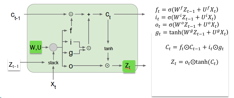
Figure 13.9: Internals of a LSTM Cell

Just like RNNs, LSTMs also feature Hidden Layer nodes \(Z_t\). Using \(Z_{t-1}\) and the input \(X_t\), the Cell generates the next set of Hidden Layer values \(Z_t\). However, LSTMs are different from RNNs in the following ways:

• The fundamental difference between LSTMs and RNNs is the presence of the Cell Memory \(C_t\) in the former. The LSTM Cell operates on the Cell Memory \(C_{t-1}\) from the previous stage, and generates the next Cell Memory \(C_t\). As explained below, the Cell Memory values change by using componentwise addition and subtraction rather than matrix multiplication. Also the new Cell Memory \(C_t\) is used to generate the next Hidden State \(Z_t\).
• Another difference is the extensive use of gates in LSTMs. Indeed the vectors \(f_t, i_t\) and \(o_t\) are all used to generate gating values that regulate the flow of data in the LSTM Cell. In turn, \(f_t, i_t\) and \(o_t\) are computed using three new pairs of weight parameter matrices \((W^f,U^f), (W^i,U^i)\) and \((W^o,U^o)\) respectively.

The equations that describe the operations in a LSTM Cell are as follows (note that the symbol \(\odot\) denotes componentwise multiplication in all these equations):

• Gate Computations:
  • Compute Input Gate: \[\begin{equation} i_t = \sigma(W^i X_t + U^i Z_{t-1}) \tag{13.6} \end{equation}\]
  • Compute Forget Gate: \[\begin{equation} f_t = \sigma(W^f X_t + U^f Z_{t-1}) \tag{13.7} \end{equation}\]
  • Compute Output/Exposure Gate: \[\begin{equation} o_t = \sigma(W^o X_t + U^o Z_{t-1}) \tag{13.8} \end{equation}\] Note that in all these formulae, the function \(\sigma\) is applied on a componentwise basis.
• Update Cell Memory Value
  • Compute contribution to Cell Memory from current state \(X_t\) while taking the contribution from the previous Hidden State \(Z_{t-1}\) into account: \[\begin{equation} {\tilde C}_t = \tanh(W^g X_t + U^g Z_{t-1}) \tag{13.9} \end{equation}\]
  • Combine contribution from current state \(\tilde C_t\) with old memory \(C_{t-1}\) to get new memory \(C_t\) using the gating functions \(f_t\) and \(i_t\): \[\begin{equation} C_t = f_t\odot C_{t-1} + i_t\odot{\tilde C_t} \tag{13.10} \end{equation}\]
• Compute the new Hidden State vector using the new memory \(C_t\) and the gating function \(o_t\): \[\begin{equation} Z_t = o_t\odot\tanh(C_t) \tag{13.11} \end{equation}\]

In order to get an intuitive understanding of these equations, assume the following:

• The sigmoid function acts as a 1-0 switch. so that \(i_t, f_t\) and \(o_t\) only take values of \(0\) or \(1\).
• The tanh function acts a \({+1,-1}\) switch, so that \({\tilde C}_t\) only takes values of \(+1\) or \(-1\).

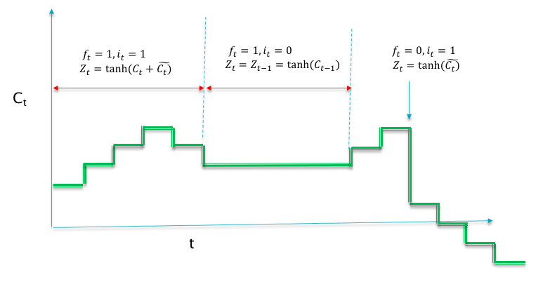
Figure 13.10: Time Evolution of a Component of the LSTM Cell State

Under these assumptions, a typical trajectory of one of the components of the Cell State vector \(C_t\) is shown in Figure 13.10. In this simplified system, one can clearly see that the Cell State \(C_t\) exhibits four kinds of behaviors (see Equation (13.10)):

1. \(C_t\) changes in value in response to new inputs \(X_t\): This happens when \(i_t = f_t = 1\), and the cell state increments or decrements by \(1\) at each time step.
2. \(C_t\) holds the old value from the previous stage: This happens when \(i_t =0, f_t = 1\), and results in \(C_t = C_{t-1}\).
3. \(C_t\) resets to the value \(\tilde C_t\): This happens when \(i_t =1, f_t = 0\) and results in \(C_t = \tilde C_t = \tanh(W^g X_t + U^g Z_{t-1})\). Note that this is not a complete reset, since the prior history is still be propagated through \(Z_{t-1}\).
4. \(C_t\) resets to zero: This happens when \(i_t =0, f_t = 0\) and results in a complete reset.

Since the output of the system is a function not of cell state \(C_t\) but the Hidden State values \(Z_t\), it is important to examine its behavior as well. Each component of \(Z_t\) vector takes on values from the set \(\{+1,0,-1\}\) and from Equation (13.11) one can see that:

1. Changes in value in response to new inputs \(X_t\): This happens when \(i_t = f_t = o_t = 1\). Note that \(Z_t = \tanh(C_{t-1} +\tilde C_t)\) can potentially flip between \(+1\) and \(-1\) in response to changes in \(C_t\) (or vary continuously if it is in the linear portion of the tanh curve).
2. Holds the old value from the previous stage: This happens when \(i_t =0, f_t = 1, o_t = 1\), and results in \(Z_t = Z_{t-1}\).
3. Resets to the (tanh) value of the new cell state: This happens when \(i_t =1, f_t = 0, o_t = 1\) and results in \(Z_t = \tanh(\tilde C_t)) = \tanh(\tanh(W^g X_t + U^g Z_{t-1}))\). Note that \(Z_t\) still retains memory of the prior state, hence it is not a complete reset.
4. Resets to zero: This happens when \(o_t = 0\) or when \(i_t =0, f_t = 0\) and results in \(Z_t = 0\), resulting in a full reset.

At each stage, the vector of \(+1\) and \(-1\) values belonging to the Hidden State \(Z_t\), are converted to the logit values \(A^Y\) by using the linear transform \[ a_k^Y = \sum_{j=1}^P a^Y_{kj} z_j + b^Y_k, \quad 1\le k\le K \]

Figure 13.11: Interpreting Cell State Values in LSTMs

From this analysis it is clear that LSTMs are much more effective in retaining memory of past inputs as compared to RNNs. Indeed it is possible for LSTMs to propagate a state value indefinitly into the future by setting the gates \(f_t = 1, i_t = 0\), as the analysis shows. An example of this is shown in Figure 13.11 which shows the value of a single component of the Cell State vector in a LSTM system that was trained to generate sentences in English (this system is described later in this chapter). This cell state component was in the ON state (shown in blue) whenever the system is generating characters that lie in between quotes, and is OFF otherwise (shown in red). This illustrates the LSTMs ability to change its state and hold it in response to the input values.

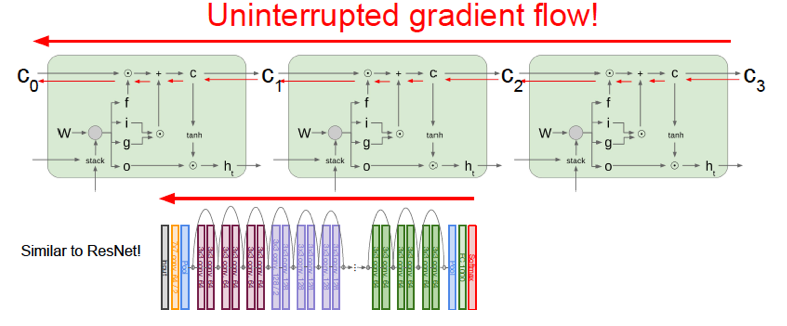
Figure 13.12: Gradient Flow in LSTMs

LSTMs derive a lot of their modeling power from the fact that they provide a way in which the gradients can flow backward, using componentwise additive and multiplicative operations, rather than matrix multiplications (see Figure 13.12). The red arrows show the gradients with respect to the cell states flowing back. The addition gate passes them on unchanged, while the multiplication gate \(f\) resets them to zero or passes them on unchanged (assuming that takes \(f\) on values \(0\) or \(1\)). Furthermore the error value \(y-t\) modify the gradients with respect to the cell state \(C\) at each stage, and these modifications are able to propagate all the way back unimpeded.

There is an interesting similarity between LSTMs and the best performing ConvNet architecture called ResNets (see Chapter 12), since both feature the additive interaction design. Not all aspects of why this is beneficial are understood at this point, and this topic forms an active area of research.

13.5 Gated Recurrent Units (GRUs)

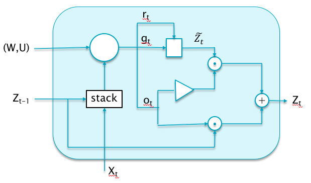
Figure 13.13: Gated Recurrent Units (GRUs)

GRUs are a recently proposed alternative to LSTMs, that share its good properties, i.e., they are also designed to avoid the Vanishing Gradient problem (see Figure 13.13). Even though they feature fewer parameters than LSTMs, their performance has been experimentally seen to be about the same. The main difference from LSTMs is that GRUs don’t have a cell memory state \(C_t\), but instead are able to function effectively using the Hidden State \(Z_t\) alone.

The design of the GRU features two gates, the Update Gate \(o_t\), given by: \[\begin{equation} o_t = \sigma(W^o X_t + U^o Z_{t-1} \tag{13.12} \end{equation}\] and the Reset Gate \(r_t\) given by: \[\begin{equation} r_t = \sigma(W^r X_t + U^r Z_{t-1} \tag{13.13} \end{equation}\] The Hidden State vector \(Z_{t-1}\) from the prior stage is combined with the Input vector \(X_t\) from the current stage, to generate an intermediate Hidden State value \(\tilde Z_t\) given by: \[\begin{equation} {\tilde Z}_t = \tanh(r_t\odot U Z_{t-1} + W X_t) \tag{13.14} \end{equation}\] Finally the new Hidden State \(Z_t\) is generated by combining the prior Hidden State \(Z_{t-1}\) with the intermediate value \(\tilde Z_t\) as follows: \[\begin{equation} Z_t = (1 - o_t)\odot {\tilde Z}_t + o_t\odot Z_{t-1} \tag{13.15} \end{equation}\]

In order to understand the workings of the GRU, we once again assume that both the Update and Reset gates are operating in the saturated regime, so that they assume values in the set \(\{0,1\}\). It is easy to see that each component of \(Z_t\) vector takes on values from the set \(\{+1,0,-1\}\) and from Equtions (13.14) and (13.15) one can see that it can exhibit the following behaviors:

1. It changes in value in response to new inputs \(X_t\): This happens when \(o_t = 0, r_t = 1\), and \(Z_t = \tilde Z_t = \tanh(U Z_{t-1} + W X_t)\). \(Z_t\) can potentially flip between \(+1\) and \(-1\) in response to changes in \(X_t\) (or vary continuously if it is in the linear portion of the tanh curve).
2. It holds the old value from the previous stage: This happens when \(o_t = 1\), and results in \(Z_t = Z_{t-1}\).
3. It resets to the value of the new input: This happens when \(o_t = 0, r_t = 0\) and results in \(Z_t = \tilde Z_t = \tanh(W X_t)\). Note that this is a full reset since all memory of prior states is lost.

The reader will notice that there are similarities in the behavior of \(Z_t\) in GRUs and LSTMs, in the sense both have modes in which \(Z_t\) maintains its prior value as well, as well as modes in which it changes value based on current input or gets reset and looses memory of prior states. However GRUs are able to do this using a smaller number of parameters. The GRU design also provides a path for the gradients with respect to \(Z\) to flow backwards without being subject to matrix multiplication, as an application of the Gradient Flow rules to Figure 13.13 reveals. This gradient flow is gated by \(o_t\), such that if \(o_t = 0\) at a cell, then the gradient is not propagated backwards.

13.6 Applications of RNNs

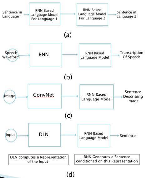
Figure 13.14: Some Applications of RNNs

RNNs have been successfully used to solve problems in the following areas (note that in the rest of this chapter whenever we refer to RNNs, we are also implicitly referring to other recurrent models such as LSTMs and GRUs):

• Machine Translation
• Speech Transcription
• Image Captioning
• Parsing
• Handwriting Recognition
• Information Retrieval
• Chatbot desgn

Figure 13.14 shows the high level architecture of several systems of practical importance that utilize RNNs. As Part (d) of the figure illustrates, these systems consist of two parts:

• Part 1 consists of a DLN model whose job is to process the Input and create a high level representation for it. This can be done using any one of the DLNs that we have discussed in this book, namely Fully Connected Feed Forward networks, ConvNets or RNNs.
• Part 2 consists of a Language model, which is built using RNNs.

The function of the Language Model is to generate a sentence in a target language, by using the context provided by the DLN based representation from Part 1. Parts (a)-(c) of Figure 13.14 show some examples of this:

• Part (a) of the figure shows the case when the system is used for doing Machine Translation. The input is a sentence in Language 1, which is converted into a vector representation using a RNN. This representation is then fed into the Language Model which outputs a translation in Language 2.
• Part (b) of the figure shows the case when the system is used to convert a speech sound waveform into a sentence. It uses a RNN for obtaining a vector representation for the waveform which is then fed into the Language Model that generates the corresponding words.
• Part (c) of the figure shows the case when the system is used to generate captions for images. The image is first converted into a high level representation using a ConvNet, followed by the Language Model that generates the caption.

Since several important applications of RNNs involve Language Modeling, we look at this topic in more detail in the next sub-section. In the following sub-section we consider Encoder-Decoder Architectures that are used to implement the end-to-end systems of the type shown in Figure13.14.

13.6.1 RNN Based Language Models (RNN-LM)

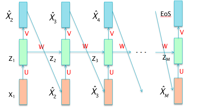
Figure 13.15: Language Modeling using RNNs

Language Modeling is the process of designing models that are capable of generating sentences that have a high probability of actually occuring in the target language. Lets assume that the Language Model generates a sentence consisting of Q words \((X_1,...,X_Q)\) such that the \(i^{th}\) word is represented by the vector \(X_i\). The probability of the occurrence of this sentence is given by \(p(X_1,...,X_Q)\). Using the Law of Conditional Probabilities it follows that \[ p(X_1,...,X_Q) = \prod_{i=1}^Q p(X_i|X_1,...,X_{i-1}) \] This implies that the probability of the sentence can be computed by finding the conditional probabilities \(p(X_i|X_1,...,X_{i-1}), i=2,...,Q\). This is a very important result, since it has two implications:

• Not only can the above equation be used to compute the probability of the occurrence of a sentence, it can also be used to actually generate the sentence. This is done by reducing the problem of generating a sentence consisting of \(Q\) words to solving \(Q\) successive classification problems. This is good news, since we casn now apply the machinery of Neural Networks to solve this problem.

• Due to the form of the classification required, i.e., the computation of the conditional probability \(p(X_i|X_1,...,X_{i-1})\), the problem fits in neatly within the purview of RNN models.

Making use of this equation results in a RNN model that can be used to generate sentences, known as a RNN-LM (see Figure 13.15. In this network, the first word \(X_1\) serves as the input to the first stage, while the subsequent inputs are chosen to be the outputs from the prior stage. The conditional probabilties are computed using the RNN

\[ P(X_i = w|X_1,...,X_{i-1}) = h_w(V(Z_i)) \] where \(h_w\) is the probability that the output word is \(w\), as given by the softmax function. The Hidden State \(Z_i\) captures the effect of all the preceding words \((X_1,...,X_{i-1})\) in the sentence.

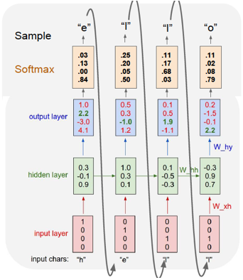
Figure 13.16: A Character Level Language Model

Using exactly the same techniques, RNN-LMs can also be trained using characters rather than words,as shown in Figure 13.16. This figure shows the generation of the word “hello” using a RNN-LM with four stages. Each of the characters ‘h’, ‘e’, ‘l’ and ‘o’ are coded using the vectors \((1,0,0,0), (0,1,0,0), (0,0,1,0)\) and \((0,0,0,1)\) respectively. The character ‘h’ is used as input into the first stage of the RNN, and results in the output probabilities shown. This output clearly does not correspond to the correct output ‘e’, hence the difference between the two is used to generate the error signal during backpropagation. The second stage is then fed with the correct letter ‘e’, and the training process continues until we get to the last stage.

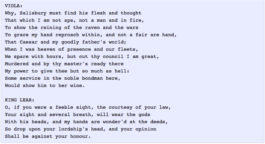
Figure 13.17: Output of a RNN-LM Trained on the Works of Shakespeare

RNN-LMs can be used to generate sample sentences from the corpus on which they have been trained. As an example, Figure 13.17 shows the output of a character level RNN-LM model that was trained on the complete works of William Shakespeare. As the reader may notice that even though the sentences themselves are nonsensical, they are gramatically correct and use valid English words. Also the RNN has learnt the names of characters in the play, that it has affixed them correctly before the start of each dialog.

As alluded to at the start of this section, the power of the RNN-LM model formulation is realized when they it is used to generate Conditional Language, which is defined as sentences that are generated in response to an additional input, such as an image, a video clip or a sentence in another language. This results in an image caption, a video description and a translation respectively. In Section 13.6.2 we introduce Encoder Decoder Architectures that are used to realize this vision.

There are two other techniques that have proven to be very useful when building Language Models, namely Word Embeddings and Beam Search, and these are briefly described next.

13.6.1.1 Word Embeddings

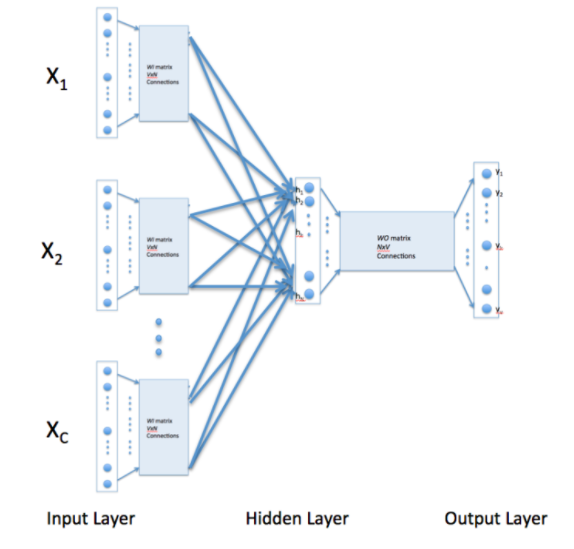
Figure 13.18: Continous Bag of Words (CBOW) Model

The coding rule used to encode words in a corpus is known as Word Embedding and it is used to convert the vocabulary of words into points in a high dimensional co-ordinate space. The most straightforward rule is called 1 of K Encoding (also known as One-Hot Encoding), and works as follows: If the vocabulary under consideration consists of a certain number of words, say 20,000 words, then the system encodes them using a 20,000 dimensional vector, in which all the co-ordinates are zero, except for the identifying co-ordinate, that is set one. Thus each word is identified by the unique position of its corresponding co-ordinate.

There are two problems with 1 of K Encoding schemes:

• It results in extremely high dimensional input vectors, and the dimension increases with increasing number of words in the vocabulary.
• The coding scheme does not incorporate any semantic information about the words, they are all located equi-distant from each other at the vertices of a K-dimensional cube.

In order to remedy these problems, researchers have come up with several alternative algorithms to do Word Embeddings. The most popular way of representing words in vector form requires just a few hundred dimensions, and is implemented as part of the popular Word2Vec algorithm. This representation is created by using the words that occur frequently in the neighborhood of the target word, and it has been shown to capture many linguistic regularities.

Word2Vec uses two algorithms to generate Word Embeddings, namely Continuous Bag of Words (CBOW) and Skip-Gram. Both these algorithms use shallow DLNs that are trained in an unsupervised manner, so they are extremely fast. Figure 13.18 shows the CBOW network, and it works as follows: The Input Layer consists of 1 of K encoded representations for all the words, except one, in a sentence belonging to the training corpus. The main idea of the algorithm is to train the network to generate the missing word, and then use the rows of the \(V\times N\) weight matrix \(WI\) as the embeddings (\(V\) is the number of words on the vocabulary and \(N\) is the dimension of the Embedded Words). The network basically compresses the \(V\) dimensions of the input word into \(N\) dimensions, and then de-compresses it using a \(N\times V\) matrix to generate the 1 of K output vector corresponding to the missing word. If there are \(nb(t)\) words being associated with the target word \(w_t\), then the following Loss Function is used to train the network:

\[ L = -{1\over V}\sum_{t=1}^V\sum_{j\in nb(t)} \log p(w_j|w_t) \] In this equation \(w_j\) is the set of neighborhood words that occur in association with \(w_t\) in the corpus.

In general words that are semantically close to each other tend to cluster together in the embedded space. As an example, consider the following vector operation which makes use of Word Embeddings (vec(‘x’) stands for the Word Embedding representation for the word ‘x’): \[ vec('Paris') - vec('France') + vec('Italy') = vec('Rome') \] Hence Word Embeddings incorporate the meaning of word into their representations, which gives better results when these vectors used in various operations involving words and language.

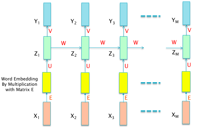
Figure 13.19: Using Word Embeddings in RNNs

Figure 13.19 shows how Word Embeddings are used in RNN models. The inputs \(X_i\) are encoded using 1 of K encoding, and then multiplied by the embedding matrix \(E\) which converts them into their embedded representation. These are then fed into the rest of the RNN.

13.6.1.2 Beam Search

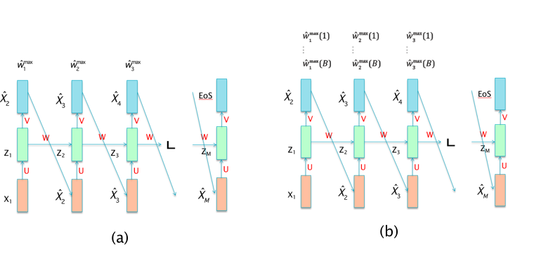
Figure 13.20: (a) Greedy Search, (b) Beam Search

The Beam Search technique was invented back in the 1970s with the first Machine Translation systems, and is used to solve the problem of choosing the best output sequence in RNN-LM models. Beam Search proceeds as follows: During the prediction part of the algorithm, when the system gets to the step that generates the first predicted output vector \({\hat X}_2\), it actually assigns probabilities \(p_2^k, 1\le k\le K\) for all the \(K\) words in the output alphabet. The algorithm can then choose to either:

• Choose \({\hat X}_2\) to be the ouput vector \(k\) for which \(p_2^k\) is the largest, and then feed this vector as the input in the next step for predicting \({\hat X}_3\). This is known as Greedy Search and is shown in Part (a) of Figure 13.20.

• Instead of choosing a single vector, we choose the \(B\) vectors \((p_2^{k1},...,p_2^{kB})\) whose output probabilities are the largest. Each one of these \(B\) vectors is then fed as the input at the next step, resulting in a total \(B^2\) candidate vectors at the end of the second stage. However this list is then pruned back to size \(B\) by choosing the \(B\) vectors for whom the product \(p_2^{ki}p_3^{kj}\) is largest. These vectors are then fed as the input into the third step, and the process continues. This is known as Beam Search and is shown in Part (b) of Figure 13.20.

13.6.2 Encoder-Decoder Systems

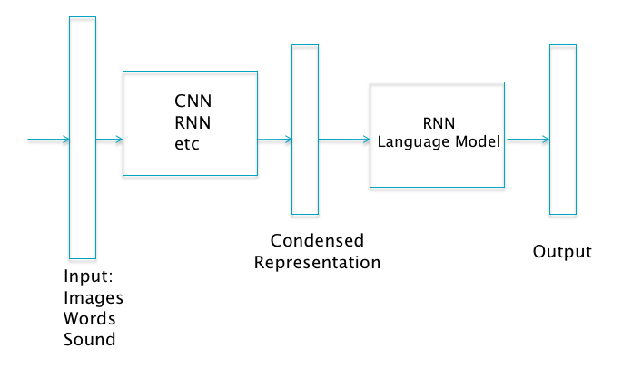
Figure 13.21: Encoder Decoder System

In the next few sub-sections we describe Encoder-Decoder architectures of the type shown in Figure 13.21. These systems are created by coupling a RNN based Language Model with a DLN that computes a representation for the input data. Almost all the important applications of RNNs fall within this class of models. Before we do so, we discuss a technique called Attention Mechanism that is commonly used in Encoder-Decoder systems.

13.6.2.1 The Attention Mechanism

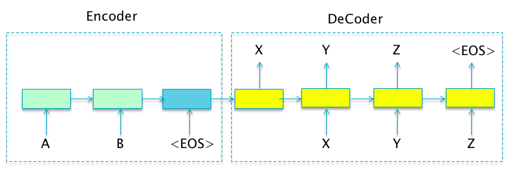
Figure 13.22: Sequence to Sequence Learning

Attention Mechanism is a recently discovered technique that has already had a big impact in improving the performance of Encoder-Decoder systems. In order to justify the reason why its needed, lets consider the example of Sequence-to-Sequence Learning systems of the type shown in Figure 13.22. The figure shows an Encoder made up of a two stage RNN. The final Hidden Layer in the Encoder is fed into the Decoder, which is a RNN-LM with four stages. The system takes an input sequence AB and maps it to an output word sequence XYZ. A central premise of this architecture is that the system is able to compress sufficient information about the variable size Input Sequence within the final Hidden State of the Encoder part of the network. This Hidden State is then used to generate the entire Output Sequence without any further assistance from the Encoder. However, as the Input Sequence grows, it begs the question of how efficiently can variable size input information be captured within a fixed number of hidden nodes. In practice it has been observed that as the size of the Input Sequence grows, especially if it is larger than the size of the sentences in the Training Data, the performance of the system detoriates rapidly. This points to an architectural weakness, which needs to be addressed.

The Attention Mechanism was designed to address this issue. It enables the decoder to focus on specific portions of the encoder while doing the decoding. For the special case of Sequence-to-Sequence Learning, the Attention Mechanism operates as follows: Each time the Decoder generates a word, it uses its current Hidden State as context to (soft) search the entire set of Encoder Hidden States for a set of vectors that have the most relevant information for generating the next output word. These vectors are then used to create a special vector called the Context Vector, which is then used to predict the next output word based on the Encoder information, as well all the previously generated output words. As a result the system is not forced to compress all the information in the Input Sequence, irrespective of its length, into a fixed length vector.

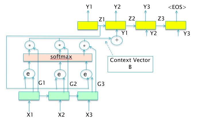
Figure 13.23: The Attention Mechanism

We now formalize these ideas for the case of a general Encoder Decoder Network (see Figure 13.23).

• Choose a structured representation of the Input, which is referred to as the Context Set. This will denoted by a set of vectors \(G\)

\[ G = \{G_1,...,G_{L_{in}}\} \] Each of these vectors contains summary information about a localized region of the input (spatial, temporal or spatio-temporal). Examples: If the input is an image, then \(G_i\) encodes information about a certain spatial location on the image, in the case of sequence to sequence learning/machine translation systems, \(G_i\) encodes information about the words centered around a specific word in the input sentence.

• The Attention Mechanism controls the portion of the input actually seen by the Decoder, and this is achieved by means another DLN \(f_{ATT}\) which is referred at as the “Attention Model”. The Attention Model scores each Contex Vector \(G_i\) with respect to the current Decoder Hidden State \(Z_{t-1}\) by an Attention Score \(e_i^t\), using the following model: \[\begin{equation} e_i^t = f_{ATT}(Z_{t-1}, G_i, \{ \alpha_j^{t-1} \}_{j=1}^{L_{in}}) \tag{13.16} \end{equation}\] where the sequence \(\alpha_j^t\) represents the Attention Weights computed from the Attention Scores \(e_i^t\), and is given by \[\begin{equation} \alpha_i^t = \frac{e_i^t}{\sum_{j=1}^{L_{in}} e_j^t} \tag{13.17} \end{equation}\] The Attention Weight \(\alpha_i^t\) is the probability that the Decoder attends the region of the input encoded by the Context Vector \(G_i\).
• The Attention Weights are then used to compute the new Context Vector \(B_t\) given by \[ B_t = \psi(\{G_i\}_{i=1}^{L_{in}}, \{ \alpha_i^t \}_{i=1}^{L_{in}}) \] A popular choice for \(\psi\) is a simple weighted sum of the vectors in the Context Set, given by \[\begin{equation} B_t = \sum_{i=1}^{L_{in}} \alpha_i^t G_i \tag{13.16} \end{equation}\] Equation (13.16) states that the weight that the decoder attaches to the \(i^{th}\) encoder location, is a function of:
  • The hidden state value from the prior decoder stage \(Z_{t-1}\),
  • The Context Vector \(G_i\) associated with the \(i^{th}\) encoder location. This factor results in Content Based Attention, which is independent of the location \(i\) of the vector.
  • The sequence \(\{ \alpha_j^{t-1} \}_{j=1}^{L_{in}}\), which is the set of Attention Weights at the previous time instant. This factor results in Location Based Attention, since if the previous set of weights is strongly peaked around some location, then the new set of weights can also be chosen to be peaked around a neighboring location.
• The Context Vector \(B_t\) is then used to update the Hidden State and Output of the Decoder, which in the case of a RNN-LM model is given by

\[\begin{equation} Z_t = f(WZ_{t-1} + UY_{t-1} + SB_t) \tag{13.18} \end{equation}\] \[\begin{equation} Y_t = h(VZ_t + U'Y_{t-1} + S'B_t) \tag{13.19} \end{equation}\]

13.6.2.2 Applications of Encoder Decoder Systems

The following applications of the Encoder-Decoder architecture are described in this section:

• Sequence to Sequence Natural Language Processing (NLP) Systems and Neural Machine Translation

• Image Captioning

• Speech Recognition

All three applications are of commercial importance, and have an extensive history of older non-neural network based algorithms that were used to solve them. In each case, Encoder-Decoder systems now either match or out-perform the older algorithms.

13.6.2.2.1 Sequence to Sequence NLP Systems

Sequence to Sequence NLP Systems constitute an important special case of the Encoder Decoder architecture and they are designed to map a variable length input word sequence \(X_i, i=1,...,L_{in}\) to a variable length output word sequence \(Y_i,i,...,L_{out}\). Since the input and output sequences may be of different lengths in general, it is not possible to use a RNN architecture of the type shown in Figure 13.2 which restricts the output sequence to be of the same length as the input sequence.

One way to solve this problem is shown in Figure 13.22. In this architecture,the RNN is split into two parts:

• The sequence of input words \(\{A,B\}\) is processed by the Encoder and the information in the sequence is summarized in the final hidden state. Note that during the time the input sequence is being processed, the system does not emit any output.

• The Decoder part of the system uses the information in the final hidden state of the Encoder to create the output word sequence \(\{X,Y,Z\}\) using a RNN-LM system.

There are a number of commercially important applications for this system, including:

• Language Translation: The input corresponds to a sentence from Language A and the output is its translation into Language B.
• Document Summarization: The input corresponds to the words in a document and the output is a shorter summary of its content.
• Email Auto-Reply: The input corresponds to the contents of an email and the output is the appropriate reply to that email.
• Conversation or Q&A: The input corresponds to words of a conversation (or a question), and the output contains the words of an appropriate response.

We now describe an important sub-case of Sequence to Sequence NLP systems that are used to do Machine Translation.

13.6.2.2.1.1 Neural Machine Translation

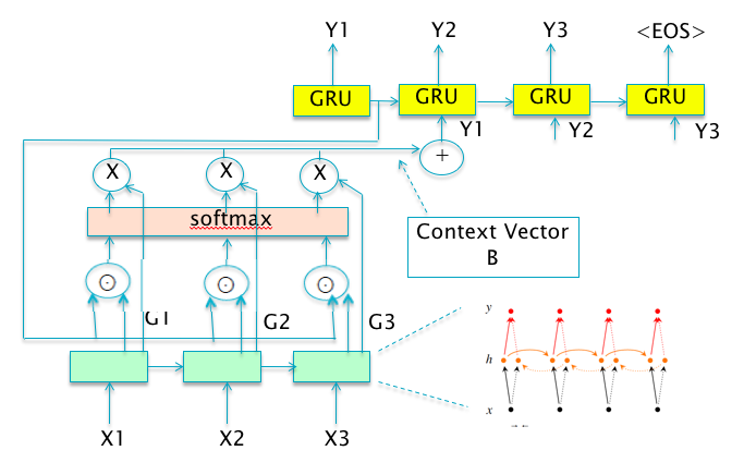
Figure 13.24: Illustration of Attention Based Neural Machine Translation

Machine Translation is the process of taking a sentence from Language A as input, and generating its translation in Language B as the output. The traditional way of doing this was a Bayesian ML algorithm called Statistical Machine Translation (SMT). However in the last two years, Neural Machine Translation (NMT) systems have surpassed SMT in their accuracy, and as a result popular websites such as Google have replaced SMT with NMT in their production systems.

In this section we start by describing a NMT system designed by Bahdanau et.al. [ ]. The system follows the general Sequence-to-Sequence Learning architecture enhanced using the Attention Mechanism as shown in Figure 13.24:

• The system uses GRUs (see Section 13.5) in place of plain RNN nodes in both the Encoder and Decoder.

• In the Encoder, the system uses a bidirectional RNN design in which one set of nodes process the input in the order \((X_1,...,X_T)\), while another set of nodes process the input in the reverse order \((X_T,...,X_1)\). This results in two sets of Hidden State Vectors: The vectors \((H_1,..,H_T)\) are created from the forward sequence of inputs, while the vectors \((H'_T,...,H'_1)\) are created from the backward input sequence. The bi-directional design ensures that the vectors in the Context Set (defined below), summarize not just the preceding words, but also the following words.

• The system incorporates the Attention Mechanism described in Section 13.6.2.1, in which the the two Hidden State vectors are concatenated together to create the vectors in the Context Set \(G_i = [H_i,H'_i]\). The Attention Scores \(e_i^t\) are then computed using the following formula:

\[ e_i^t = V_a^T \tanh(W_aZ_{t-1} + U_a G_i) \] where the vector \(V_a\) and the matrices \(W_a\) and \(U_a\) are parameters that are learnt during Backprop.

The rest of the algorithm proceeds as described in Section 13.6.2.1, with the Attention Weights computed using Equation (13.17) and the Context Vectors created using the weighted linear combination from Equation (13.16). The Decoder Hidden State is updated according to state update rules for GRUs (see Section 13.5) modified by the fact that there is an additional input corresponding to the State Vector \(G_t\).

Another NMT architecture was proposed by Sutskever et.al. [ ], whose performance is comparable to the one described above. This design also uses the basic Sequence-to-Sequence architecture from Figure 13.22, however it does not use the Attention Mechanism. Instead it uses the simple technique of reversing the Input Sequence as follows: Instead of feeding the input sequence \(\{X_1,X_2,...,X_{L_{in}-1},X_{L_{in}}\}\) in that order, the sequence is reversed and fed in the order \(\{X_{L_{in}},X_{L_{in}-1},...,X_2,X_1\}\). The intuitive justification for this rule is based on the following heuristic: When the system is being used for Language Translation then output word \(Y_1\) is most influenced by the input word \(X_1\) and perhaps others near to it. However when the input sequence is fed in the correct order, then \(X_1\) and \(Y_1\) are far apart from each other, which makes it more difficult for the system to remember \(X_1\) and use this information to come up with \(Y_1\). Hence by reversing the input sequence we bring them closer to one other, which improves the translation performance. Also the system uses four layers of LSTMs in the Encoder, instead of the Bi-Directional GRU design used by Bahdanau et.al.

13.6.2.2.2 Image Captioning

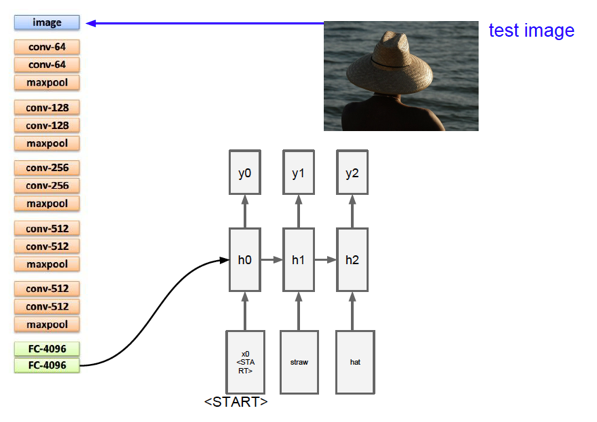
Figure 13.25: Image Captioning - Architecture 1

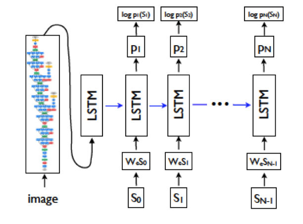
Figure 13.26: Image Captioning - Architecture 2

The Machine Translation application of the Encoder-Decoder architecture featured the same media type on both sides. In this section we describe an application in which two different media are involved: An image on the encoding side and its corresponding description (or caption) in a language such as English, on the decoding side. Creating an image description involves the following tasks:

• The description should capture the most significant objects in the image.
• It should express how these objects relate to each other, as well as their attributes and activities they are involved in.
• This semantic knowledge has to be converted into a natural language, which implies the use of a Language Model to do so.

This is an inherently difficult problem to solve, and before the advent of Encoder-Decoder systems, was typically approached by stitching together the solution for the object recognition problem and filling in pre-existing caption templates. These type of systems were rigid in their text generation, and were demonstrated to work well only in limited domains such as traffic scenes or sports. The Encoder-Decoder based solution on the other hand, was inspired by the Machine Translation systems described earlier, and uses a single joint model that takes an Image \(I\) as input, and produces a caption \(S\) that maximizes the likelihood \(p(S|I)\).

Figures 13.25 and 13.26 show two of the proposed designs for solving the problem, and we describe these next.

• In both the designs, the Encoder part of the system is implemented using a Deep Convolutional Network which is used to generate a rich representation of the input image by embedding it in a fixed-length vector. System 1 uses a VGGNet for doing the encoding, while System 2 uses the Google Inception network. In both cases, the last Fully Connected layer that precedes the final output classification or logit layer is used as the embedded image representation vector. The ConvNet is pre-trained on the image classification task before it is inserted into the Encoder-Decoder network, and then trained again end-to-end for the image captioning task.
• The fixed length vector representing the input image is fed into the Decoder part of the system in slightly different ways in Systems 1 and 2. In System 1, the image vector is fed as a bias term into the first Hidden State, while in System 2 it is fed as an input into the first Hidden State. Both these choices seem to work quite well. Note that the image is fed into the RNN only once in the beginning, which actually works better than if the image were to be fed in every step.
• In both cases the RNN was implemented using an LSTM. The input into the LSTM was chosen to be be the embedded vector for the corresponding word (see Section 13.6.1.1 for a discussion of word embeddings), while output of the LSTM is probability of occurence for all the words in the vocabulary. The first word \(S_0\) into the LSTM is a special start word and the last word \(S_N\) is a special stop word which signals the end of the sentence. Note that both the image and the words are mapped into the same space as a result of their respective embeddings (via a ConvNet for the image and the Embedding Matrix for the words).

In System 2, a Beam Search of size 20 was shown to yield the best results. Due to the limited size of the training sets available for this application, overfitting is a serious problem. However the authors of System 2 found that if the parameters of the ConvNet are initialized to a pre-trained model, such as ImageNet, then it helps a lot. A similar improvement was not observed by pre-setting the word embedding matrix.

13.6.2.2.2.1 The Attention Mechanism Applied to Image Captioning

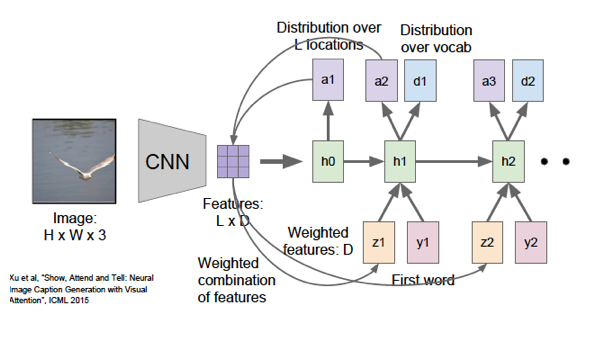
Figure 13.27: Image Captioning using Attention

Xu et.al. [ ] applied the Attention Mechanism to the Image Captioning problem and obtained excellent results with a system that they called “Show, Attend and Tell”. At a high level, the Attention Mechanism generates the caption by sequentially focusing on different parts of the image as the description progresses, and generating the word that is most relevant to the attended part (see Figure 13.28 for examples). We now go over the steps outlined in Section 13.6.2.1 that are needed to apply this algorithm. We will assume that VGGNet is the ConvNet being used to encode the image information (see Figure 13.27)..

We first need to choose the vectors in the Context Set. This is a critical design decision since it determines how the system will focus its attention on specific parts of the input image. Recall that in the two Image Captioning systems discussed earlier, the image information is conveyed by the vector formed by a Fully Connected layer in VGGNet which unfortunately doesn’t convey any local information about the image. In order to get this information, we go to the fourth Convolutional Layer (before maxpooling), which the reader may recall from Chapter 12, is a cuboid of dimensions \(14\times 14\times 512\), i.e., there are \(512\) Activation Maps, each of size \(14\times 14\). The Context Set vectors are chosen from these Activation Maps, which results in \(14\times14=196\) vectors of size \(512\) each. Each of these vectors summarizes the information from a specific region in the image, and these regions may in general overlap with one another.

The rest of the algorithm proceeds as outlined in Section 13.6.2.1: We first compute the Attention Scores using the current caption context \(Z_{t-1}\) and the portion of the image encoded by the vector \(G_i\): \[ e^t_i = f_{ATT}(G_i,Z_{t-1}) \]

We then compute the Attention Weights \(\alpha_t^i, i=1,..,512\) to be assigned to the \(i^{th}\) Context Vector when the Decoder Context is at \(Z_{t-1}\):

\[ \alpha^t_i = \frac{{e^t_i}}{\sum_{k=1}^{512} e^t_k} \] In this step we compute the resulting Context Vector \(B_t\) at Decoder step \(t\) by by doing a weighted average of all the image Context Vectors: \[ B_t = \sum_{i=1}^{512} \alpha^t_i G_i \] The system uses an LSTM in its Decoder, which results in the following state update equations:
\[ i_t = \sigma(R_i(EY_{t-1},Z_{t-1},B_t)) \] \[ f_t = \sigma(R_f(EY_{t-1},Z_{t-1},B_t)) \] \[ o_t = \sigma(R_o(EY_{t-1},Z_{t-1},B_t)) \] \[ {\tilde C}_t = \tanh(R_g(EY_{t-1},Z_{t-1},B_t)) \] \[ C_t = f_t\odot C_{t-1} + i_t\odot {\tilde C_t} \] \[ Z_t = o_t\odot \tanh(C_t) \] Finally the output \(Y_t\) of the \(t^{th}\) Decoder state is computes as: \[ Y_t = softmax[L_o(EY_{t-1} + L_z Z_t + L_b B_t)] \] Note that the matrix \(E\) in these equations is used for embedding the one-hot encoded word \(Y_{t-1}\) into a smaller state space.

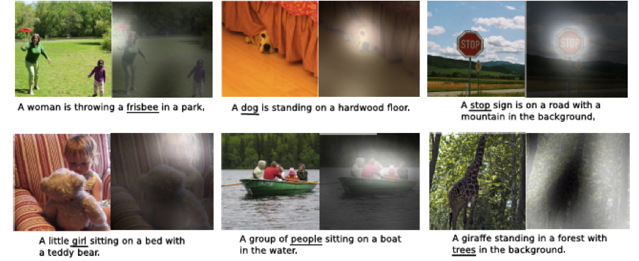
Figure 13.28: Examples of Attention Mechanism used for Captioning: The white region indicates the attended region, with the corresponding word underlined

As shown in Figure 13.28, the attention mechanism works quite well in practice. In each pair of images, the image on the left shows the area in the photo on which attention is being focussed on (by lighting up the picture in proportion to the Attention Weights). The underlined word in the generated caption is the corresponding word that was generated when attention was focussed in a particular part of the picture, and it can be seen there is a very good correspondence between the word and the image under focus.

13.6.2.2.3 Speech Transcription

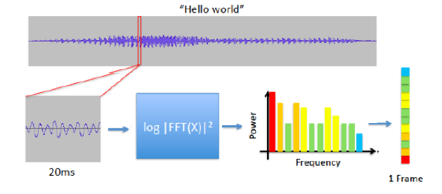
Figure 13.29: Converting Speech Waveform into Input Vectors

Speech Transcription is the process of converting the sound waveform from a spoken language into words. It is a commercially important problem, for obvious reasons, and over the years a tremenduous amount of effort has gone into designing systems that can do this task well. The process by which a speech waveform is converted into vectors that can be fed into a speech recognition model is shown in Figure 13.29 and consists of the following steps:

• The speech waveform is segmented into smaller pieces of about 20 ms each.
• Each of these segments is then processed using a Fast Fourier Transform (FFT) to extract its spectral power components. These components, organized by frequency, constitute the input into speech recognition models.

The first Speech Recognition models were built in the 1970s using a generative probabilistic model called GMM-HMM (stands for Gaussian MultiMode- Hidden Markov Model). The GMM part of the model modeled the pdf of the speech feature vectors, while the HMM part modeled the sequence information. This model was fairly complex, and made a number of assumptions about the underlying probability distributions. During the late 1990s this model was replaced by a DLN-HMM model in which a feed-forward DLN was used instead of the GMM. This led to an improvement in performance, and also allowed the system to start using less processed input signals.

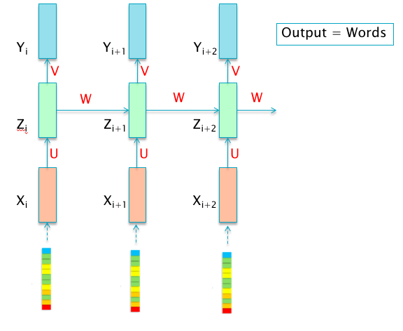
Figure 13.30: Processing Speech using RNNs

Speech Transcription can also be classified as a Pattern Recognition problem, however the patterns now occur in time rather than over space. From this point of view, RNNs are the perfect tool to solve the Speech Transcription problem since they are designed to recognize patterns in sequences that occur in time. Figure 13.30 shows a RNN based speech recognition model with speech samples as its input. The application of RNNs to this problem did not work initially for the following two reasons:

• The difficulty in training RNNs.

• Speech Transcription systems exhibit a big difference in the input and the output sequence sizes. This is due to the fact that the input sequence consists of vectors generated from filtered features of the audio waveform, which may be generated every 10 or 20 ms; while the corresponding output sequence may consist of just a few words (as can be seen from Figure 13.30). Until recently RNN architectures could not handle this disparity in input and output sequence sizes.

Both of these problems have been solved in recent years: The training problem was solved with the use of LSTMs and GRUs, while the sequence mis-match problam was solved by using the Encoder-Decoder RNN architecture since they are designed to handle inputs and output sequences of differing lengths. At this point we should also mention another RNN architecture called Connectionist Temporal Classification (CTC) that was proposed in the mid-2000s to solve the sequence mismatch problem. CTC works by using a RNN of the type in Part 5 of Figure 13.3, in which there is an output vector for every input vector. The input vector corresponds to the co-efficients of the power spectra of the sound wave (sampled every 10 or 20 ms), while the output is a corresponding letter or phenome. CTC then uses statistical techniques and language models to put together the most likely words from this data. CTC works quite well, and is widely deployed in production speech recognitions systems.

In this section we describe an alternative architecture based on the Encoder-Decoder model which was discovered more recently, and works as well as the CTC model. The system we will describe was designed by the Google Brain team which they call Listen, Attend and Spell (LAS) (see Figure 13.31). This model does not make any assumption about the nature of the probability distribution of the output character sequence, given the input acoustic sequence. Furthermore, unlike the older models, all aspects of the speech recognition system, including acoustic, pronunciation and language models, are captured within a single framework. This system learns to transcribe an audio signal into a word sequence, one character at a time, and is based on the Sequence-to-Sequence Learning framework with Attention. The Encoder part of the system is called a Listener, and the Decoder part is called a Speller and these are described next.

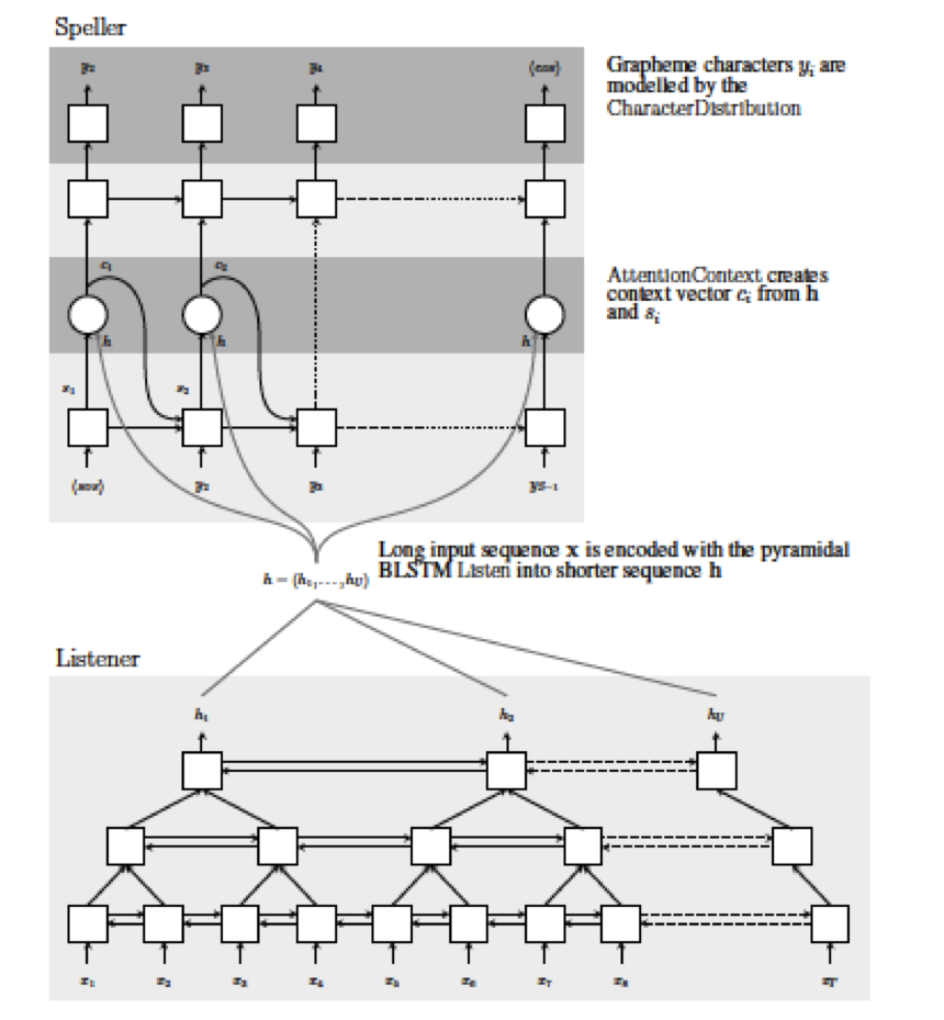
Figure 13.31: The “Listen, Attend and Spell” Model

The Listen Subsystem: The Listen system uses a Bi-directional LSTM (BLSTM) with a pyramidal structure and encodes speech signals into higher level representations (see bottom half of Figure 13.31). The reason for using this design is the following: Unlike other Encoder-Decoder systems, Speech Recognition systems exhibit a big difference in the input and the output sequence sizes due to the sequence mismatch problem. The Google Brain team observed that if the Encoder-Decoder architecture is implemented without the pyramidal structure, then it converges slowly and produced inferior results even after a training period lasting one month. This may be due to the fact that the Decoder system finds it difficult to extract the relevant information from the large number of input steps. The pyramidal BLSTM addresses this problem by reducing the time resoluton by a factor of 2 with each layer. Since the Encoder uses a 4 layer stack, it reduces the time resolution by a factor of 8 which allows the Attention Model to extract the relevant information from a smaller number of time steps.

The Attend and Spell Subsystem: At each step, the Speller uses it hidden state \(Z_t\) to guide an Attention Mechanism to compute a Context Vector \(B_t\) from the Listener’s encoded higher level features \(\{G_1,...,G_{L_{in}}\}\) which are set to the top level Hidden State vector (see top half of Figure 13.31). \[ B_t = AttentionContext(Z_t,G_1,...,G_{L_{in}}) \] The details of the AttentionContext function are as described in the Section 13.6.2.1. It then uses this Context Vector to update its internal state as well as to predict the next character in the output sequence. \[ Z_{t+1} = RNN(Z_{t},Y_{t},B_{t}) \] The next character is generated using a feed-forward DLN system as per \[ Y_{t+1} = softmax(DLN(Z_{t+1},B_{t+1})) \]

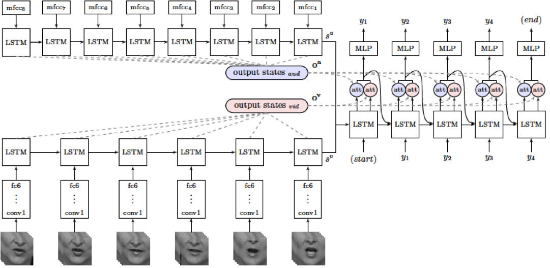
Figure 13.32: Incorporation of Lip Reading into Speech Recognition: The Listen, Watch, Attend and Spell System

A recent paper has extended the “Listen, Attend and Spell”" model to a system that also incorporates lip reading (see Figure 13.32). This system, called “Listen, Watch, Attend and Spell” has two Encoders feeding the Decoder: Encoder 1 (called “Listen”) processes the sound waveform and produces the sound Context Set vectors \(o^s\). The new Encoder 2 (called “Watch”) processes a video of the person talking. The Watch system consists of a ConvNet module based on VGGNet that generates image features for every input time step. These are then fed into a LSTM that produces the video Context Set vectors \(o^v\). The Spell module then uses an Attention model that combines the information in both sound and video Context Sets, as shown in the figure. This system is capable of operating with just the Listen module, or with just the Watch module, or with both these modules. Indeed the researchers discovered that the output word error rate decreased significantly when the Watch module was used in addition to the Listen module. Also the Lip Reading performance with only the Watch module in operation, surpassed the performance of professional lip readers.

13.7 Incorporation of Memory into DLN Architectures

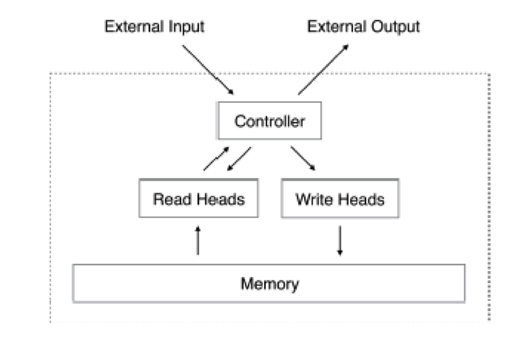
Figure 13.33: Incorporating Expicit Memory into DLNs

RNN architectures capture information about temporal patterns in the input sequence, which is then stored in a distributed fashion within its hidden states. However the system can not store or retrieve explicit information, such as the Short Memory facility in biological brains. There has been some progress in addressing this, using the architecture shown in Figure 13.33, which operates as follows: During each cycle, the controller receives an input from its internal memory and at the same time it also reads from the external memory. It then combines the input and the information read from the memory to emit a response. It may also write to the external memory during the cycle. Different architectures differ in the way the controller is designed, and it may be built for either a regular Feed Forward DLN, or a RNN. They also differ in the way the memory is accessed, either for read or write operations.

The main problem in incorporating memory into Neural Networks is the issue of addressing. If the memory is addressed explicitly, then the overall system is no longer differentiable, so is not amenable to optimization using Backprop. The architectures that have been proposed so far get around this problem by using soft addresing, i.e., instead of explicit memory locations, they access ALL of the memory during each cycle, using an Attention based mechanism that assigns probabilities of being accessed to each momory location. Hence this becomes an Associative Memory architecture, in which we access memory using the contents rather than the address of the location. Memory access is a novel application of the Attention Mechanism. It was used previously to focus on specific parts of an image (for captioning) or a single sentence (for translation), whereas in this case it is being used to focus on parts of a database consisting of multiple sentences.

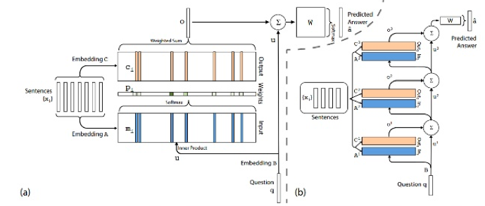
Figure 13.34: End-to-End Memory Networks

Figure 13.35: The Question-Answer Task

We now briefly describe one of the proposed architectures, called the End-to-End Memory Network (see Figure 13.34). This system is designed to store a series of statements in its memory (see Figure 13.35 for examples). The input consists of a Question, and the output is the corresponding answer as a function of the statements in memory. The system operates as follows, with reference to Part(a) of Figure 13.34:

• A set of sentences \(\{e_1,...,e_n\}\) need to be stored in memory, each word of which is represented by one-hot vector of dimension \(V\). Each word in a sentence is converted into a \(d\) dimensional vector by multiplying it with a matrix \(A\) of dimension \(d\times V\), and then the for the simple case of a Bag of Words, the representation for the entire sentence \(m_i\) is obtained by adding up the vectors for the individual words. The query \(q\) is also embedded using another a matrix \(B\) to obtain the internal state \(u\).

• The system computes a match between \(u\) and each of the memory vectors \(m_i\) by taking their inner product \(u^T m_i\), and then converts these nummbers into probabilities over the memory space by taking a softmax \(p_i = Softmax(u^T m_i)\).

• Each of the input sentences \(e_i\) is also embedded to create output vectors \(\{c_i\}\) by multiplying with an embedding matrix C. The Response Vector (which is the equivalent of the Context Vector in the Attention Mechanism algorithm) is then formed by using the following formula: \[ o = \sum_i p_ic_i \]

• The final prediction is given by summing up the Response and Input vectors, and passsing it through a weight matrix W of dimension \(VXd\), to create the vector \({\hat a}\), which gives the probabilities of the words in the vacabulary being the answer.

\[ {\hat a} = Softmax(W(o+u)) \]

The steps described above are repeated multiple times, as shown in Part (b) of Figure 13.34, with the output vector \(o_i+U_i\) from the \(i^{th}\) step serving as the input into the next stage. Each layer in general may have its own embedding matrices \(A_j, C_j\), and the output of the top of the memory layer is given by \(Softmax(Wo^K+u^K)\). The embedding matrices \(A_j\) and \(C_j\) can be chosen in various ways, and one simple choice is \(A_1 = A_2 = ...= A_K\) and \(C_1 = C_2 = ...=C_K\), which creates a RNN like structure.