Chapter 11 Deep Learning with Python

In this chapter we focus on implementing the same deep learning models in Python. This complements the examples presented in the previous chapter om using R for deep learning. We retain the same two examples. As we will see, the code here provides almost the same syntax but runs in Python. There are very few changes needed, but are the obvious ones for programming differences between the two languages. However, it is useful to note that TensorFlow in Python may be used without extensive knowledge of Python itself. In this sense, packages for implementing neural nets have begun to commoditize deep learning.

Here is the code in Python to fit the model and then test it. Very little programming is needed. First, we import all the required libraries.

import pylab

from keras.models import Sequential
from keras.layers import Dense, Dropout, Activation
from keras.layers.advanced_activations import LeakyReLU
from keras import backend
from keras.utils import to_categorical

11.1 Cancer Data

Next, we read in the data from the cancer data set we have seen earlier. We also structure the date to prepare it for use with TensorFlow.

#Read in data
import pandas as pd
tf_train = pd.read_csv("BreastCancer.csv")
tf_test = pd.read_csv("BreastCancer.csv")
n = len(tf_train)

X_train = tf_train.iloc[:,1:10].values
X_test = tf_test.iloc[:,1:10].values
y_train = tf_train.iloc[:,10].values
y_test = tf_test.iloc[:,10].values

idx = y_train; y_train = zeros(len(idx)); 
y_train[idx=='malignant']=1; y_train = y_train.astype(int)

idx = y_test; y_test = zeros(len(idx)); 
y_test[idx=='malignant']=1; y_test = y_test.astype(int)

Y_train = to_categorical(y_train,2)

The model is then structured. We employ a fully-conected feed-forward network with five hidden layers, each with 512 neurons, Dropout of 25 percent is applied. The node functional form used is Leaky ReLU. The model is compiled as well.

#Set up and compile the model
model = Sequential()
n_units = 512
data_dim = X_train.shape[1]

model.add(Dense(n_units, input_dim=data_dim))
model.add(LeakyReLU())
model.add(Dropout(0.25))

model.add(Dense(n_units))
model.add(LeakyReLU())
model.add(Dropout(0.25))

model.add(Dense(n_units))
model.add(LeakyReLU())
model.add(Dropout(0.25))

model.add(Dense(n_units))
model.add(LeakyReLU())
model.add(Dropout(0.25))

model.add(Dense(n_units))
model.add(LeakyReLU())
model.add(Dropout(0.25))

model.add(Dense(2))
model.add(Activation('sigmoid'))

model.compile(optimizer='rmsprop',
              loss='binary_crossentropy',
              metrics=['accuracy'])

Finally, the model is fit to the data. We use a batch size of 32, and run the model for 15 epochs.

#Fit the model
bsize = 32
model.fit(X_train, Y_train, batch_size=bsize, epochs=15, validation_split=0.0, verbose=1)

The programming object for the entire model contains all its information, i.e., the specification of the model as well as it’s fitted coefficients (weights). In the next section of code, we see how to take the model object and then apply it to the data for testing. We use the scikit-learn package to generate the confusion matrix for the fit. We also calculate the accuracy of the model, i.e., the ratio of the sum of the diagonal elements of the confusion matrix to the total of all its elements.

## OUT-SAMPLE ACCURACY
from sklearn.metrics import confusion_matrix
yhat = model.predict_classes(X_test,batch_size=bsize)
cm = confusion_matrix(y_test,yhat)
print("Confusion matrix = "); print(cm)
acc = sum(diag(cm))/sum(cm)
print("Accuracy = ",acc)

We run the code. Here is a sample of the training run. We only display the first few epochs. See Figure 11.1.

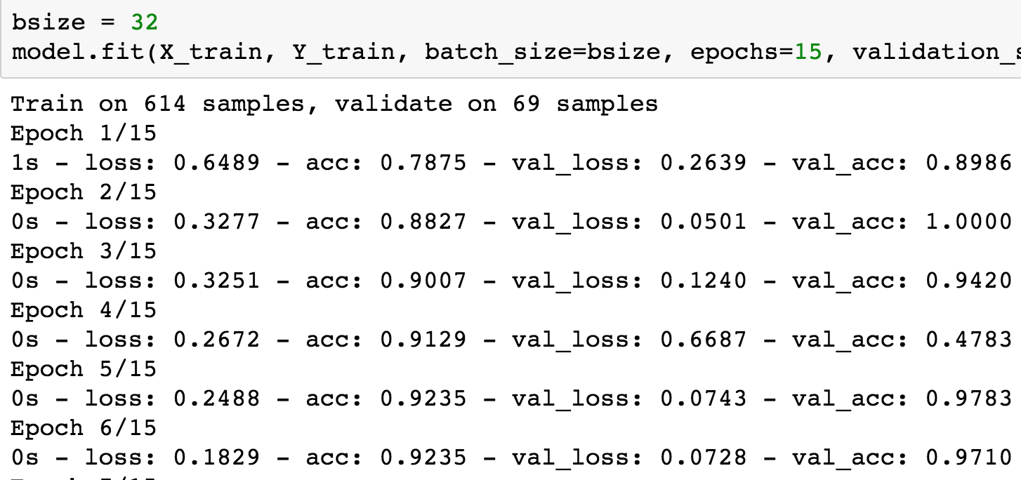
Figure 11.1: Training epochs for the cancer data set

Next, is the output from testing the fitted model, and the corresponding confusion matrix. See Figure 11.2.

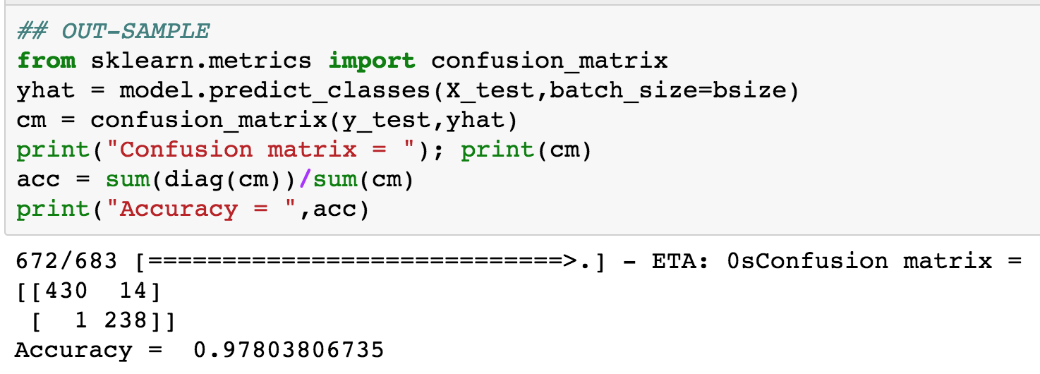
Figure 11.2: Testing epochs for the cancer data set

11.2 MNIST Data

We move on to the second canonical example, the classic MNIST data set. The data set is read in here, and formatted appropriately.

train = pd.read_csv("train.csv")
test = pd.read_csv("test.csv")

X_train = train.iloc[:,:-1].values
y_train = train.iloc[:,-1].values
X_test = test.iloc[:,:-1].values
y_test = test.iloc[:,-1].values

Y_train = to_categorical(y_train,10)

Notice that the training dataset is in the form of 3d tensors, of size \(60,000 \times 28 \times 28\). (A tensor is just a higher-dimensional matrix, usually applied to mathematica structures that are greater than two dimensions.) This is where the “tensor” moniker comes from, and the “flow” part comes from the internal representation of the calculations on a flow network from input to eventual output.

Each pixel in the data set comprises a number in the range (0,255), depending on how dark the writing in the pixel is. This is normalized to lie in the range (0,1) by dividing all values by 255. This is a minimal amount of feature engineering that makes the model run better.

X_train = X_train/255.0
X_test = X_test/255.0

Define the model in Keras as follows. Note that we have hree hidden layers of 512 nodes each. The input layer has 784 elements.

model = Sequential()
n_units = 512
data_dim = X_train.shape[1]

model.add(Dense(n_units, input_dim=data_dim))
model.add(LeakyReLU())
model.add(Dropout(0.25))

model.add(Dense(n_units))
model.add(LeakyReLU())
model.add(Dropout(0.25))

model.add(Dense(n_units))
model.add(LeakyReLU())
model.add(Dropout(0.25))

model.add(Dense(10))
model.add(Activation('softmax'))

Then, compile the model.

model.compile(optimizer='rmsprop',
              loss='categorical_crossentropy',
              metrics=['accuracy'])

Finally, fit the model. We use a batch size of 32, and 5 epochs. We also keep 10 percent of the sample for validation.

bsize = 32
model.fit(X_train, Y_train, batch_size=bsize, epochs=5, validation_split=0.1, verbose=2)

The fitting run is as follows. We see that the training and validation accuracy are similar to each other, signifying that the model is not being overfit. See Figure 11.3.

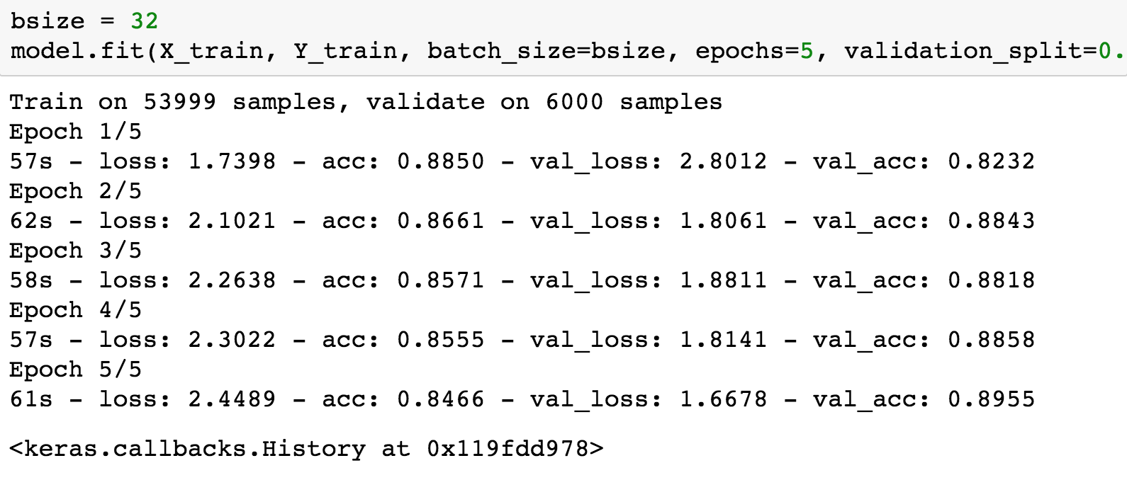
Figure 11.3: Training epochs for the MNIST data set (three hidden layers of 512 nodes each)

Here is the output from testing the fitted model, and the corresponding confusion matrix. See Figure 11.4.

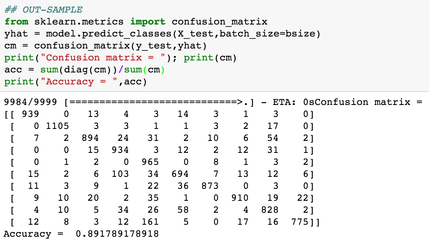
Figure 11.4: Testing epochs for the MNIST data set (three hidden layers of 512 nodes each)

The accuracy of the model is approximately 89%. We then experimented with a smaller sized model where the hidden layers only have 100 nodes each (instead of the 512 used earlier). We see a dramatic improvement in the model fit, the out-of-sample fit is shown below. Now, the accuracy is 96%. Therefore, a smaller model does, in fact, do better! Parsimony pays. See Figure 11.5.

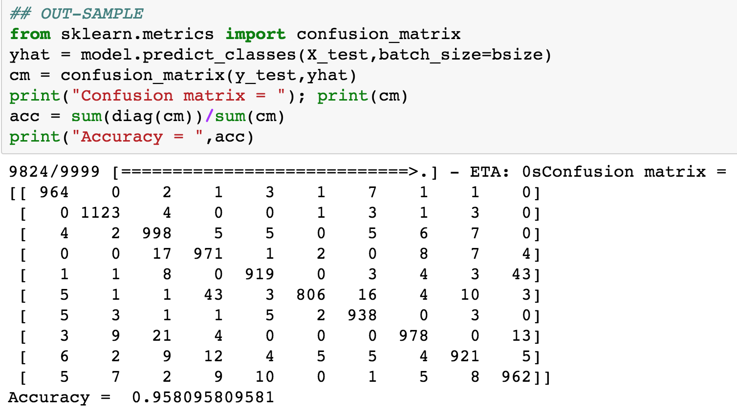
Figure 11.5: Testing epochs for the MNIST data set (three hidden layers of 100 nodes each)

11.3 Option Pricing

In a recent article, Culkin and Das (2017) showed how to train a deep learning neural network to learn to price options from data on option prices and the inputs used to produce these options prices.

In order to do this, options prices were generated using random inputs and feeding them into the well-known Black and Scholes (1973) model. The formula for call options is as follows.

\[ C = S e^{-qT} N(d_1) - K e^{-rT} N(d_2) \] where

\[ d_1 = \frac{\ln(S/K) + (r-q-0.5 \sigma^2)T}{\sigma \sqrt{T}}; \quad d_2 = d_1 - \sigma \sqrt{T} \]

and \(S\) is the current stock price, \(K\) is the option strike price, \(T\) is the option maturity, \(q\), \(r\) are the annualized dividend and risk-free rates, respectively; and \(\sigma\) is the annualized volatility, i.e., the annualized standard deviation of returns on the stock. The authors generated 300,000 call prices from randomly generated inputs (see Table 1 in Culkin and Das (2017)), and then used this large number of observations to train and test a deep learning net that was aimed to mimic the Black-Scholes equation. Here is some sample data used for training the model. The first six columns show the inputs and the last column will need to be designed to emit a positive continuous output. See Figure 11.6.

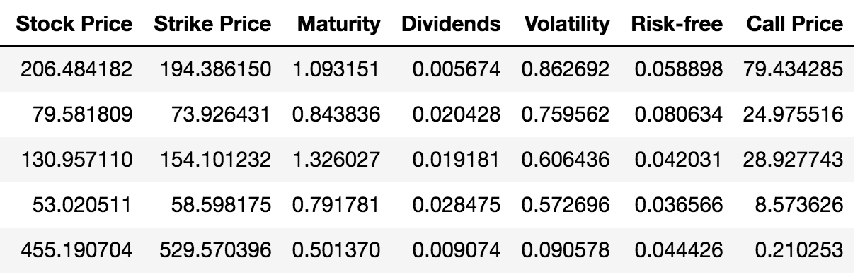
Figure 11.6: Sample data for training the deep learning option pricing model

The Black-Scholes model has the property that it is linear homogenous in the stock price \(S\) and strike price \(K\). This means that

\[ C(mS,mK) = m \cdot C(S,K) \]

This offers an excellent opportunity to normalize the data so that the level of the strike price does not play a role and this reduces the dimension of the model that needs to be fit. This means we can normalize spot and call prices and remove a variable by dividing by \(K\). \[ \frac{C(S,K)}{K} = C(S/K,1) \]

Therefore the data stored in a pandas data frame (denoted df) is normalized as follows.

## Normalize the data exploiting the fact that the BS Model is linear homogenous in S,K
df["Stock Price"] = df["Stock Price"]/df["Strike Price"]
df["Call Price"] = df["Call Price"]/df["Strike Price"]

Before feeding the data into TensorFlow, we set it up appropriately into training (\(80\%\)) and testing data (\(20\%\)) sets.

n = 300000
n_train =  (int)(0.8 * n)
train = df[0:n_train]
X_train = train[['Stock Price', 'Maturity', 'Dividends', 'Volatility', 'Risk-free']].values
y_train = train['Call Price'].values
test = df[n_train+1:n]
X_test = test[['Stock Price', 'Maturity', 'Dividends', 'Volatility', 'Risk-free']].values
y_test = test['Call Price'].values

Next, import the TensorFlow and Keras libraries.

from keras.models import Sequential
from keras.layers import Dense, Dropout, Activation, LeakyReLU
from keras import backend

Because the model aims to produce a positive continuous value for the option price, we cannot use the standard squashing functions that are used in TensorFlow, such as the sigmoid function. These functions emit values in the range \((0,1)\) and are not suitable for the range \((0,\infty)\), which is what we require. Therefore, we need to build our own output node functions, which is shown as a new python function in the following code block. The exponential function is used because it returns positive-only values

def custom_activation(x):
    return backend.exp(x)

Next, set up and compile the model. We have 4 hidden layers of 120 nodes each, and 6 input nodes and a single output node. A quick calculation shows that the total number of parameters that need to be fit for the deep learning net is \(44,407\). The code for this set up is as follows. The loss function used is mean squared error (MSE), and the optimization used the RMSprop algorithm, discussed in Section 7.3.4.

nodes = 120
model = Sequential()

model.add(Dense(nodes, input_dim=X_train.shape[1]))
model.add(LeakyReLU())
model.add(Dropout(0.25))

model.add(Dense(nodes, activation='elu'))
model.add(Dropout(0.25))

model.add(Dense(nodes, activation='relu'))
model.add(Dropout(0.25))

model.add(Dense(nodes, activation='elu'))
model.add(Dropout(0.25))

model.add(Dense(1))
model.add(Activation(custom_activation))
          
model.compile(loss='mse',optimizer='rmsprop')

We can then run the fitting method to calibrate the model by using loss function MSE. We used 10 epochs.

model.fit(X_train, y_train, batch_size=64, epochs=10, validation_split=0.1, verbose=2)

The run time shows the epochs and other metrics.

Train on 216000 samples, validate on 24000 samples
Epoch 1/10
7s - loss: 0.0049 - val_loss: 5.2774e-04
Epoch 2/10
7s - loss: 0.0014 - val_loss: 6.0296e-04
Epoch 3/10
7s - loss: 0.0010 - val_loss: 9.7482e-05
Epoch 4/10
7s - loss: 8.5638e-04 - val_loss: 9.4742e-04
Epoch 5/10
6s - loss: 7.4420e-04 - val_loss: 4.9001e-04
Epoch 6/10
6s - loss: 6.7696e-04 - val_loss: 8.6880e-04
Epoch 7/10
6s - loss: 6.3259e-04 - val_loss: 2.5829e-04
Epoch 8/10
6s - loss: 6.0162e-04 - val_loss: 1.1381e-04
Epoch 9/10
6s - loss: 5.7968e-04 - val_loss: 7.0383e-05
Epoch 10/10
7s - loss: 5.6714e-04 - val_loss: 1.3223e-04

We also define a special function to check the accuracy of the model. It generates several common statistics that we may find useful.

def CheckAccuracy(y,y_hat):
    stats = dict()
    
    stats['diff'] = y - y_hat
    
    stats['mse'] = mean(stats['diff']**2)
    print("Mean Squared Error:      ", stats['mse'])
    
    stats['rmse'] = sqrt(stats['mse'])
    print("Root Mean Squared Error: ", stats['rmse'])
    
    stats['mae'] = mean(abs(stats['diff']))
    print("Mean Absolute Error:     ", stats['mae'])
    
    stats['mpe'] = sqrt(stats['mse'])/mean(y)
    print("Mean Percent Error:      ", stats['mpe'])
    
    #plots
    mpl.rcParams['agg.path.chunksize'] = 100000
    figure(figsize=(14,10))
    plt.scatter(y, y_hat,color='black',linewidth=0.3,alpha=0.4, s=0.5)
    plt.xlabel('Actual Price',fontsize=20,fontname='Times New Roman')
    plt.ylabel('Predicted Price',fontsize=20,fontname='Times New Roman') 
    plt.show()
    
    figure(figsize=(14,10))
    plt.hist(stats['diff'], bins=50,edgecolor='black',color='white')
    plt.xlabel('Diff')
    plt.ylabel('Density')
    plt.show()
    
    return stats

We then obtain the results as follows.

y_train_hat = model.predict(X_train)
#reduce dim (240000,1) -> (240000,) to match y_train's dim
y_train_hat = squeeze(y_train_hat)
CheckAccuracy(y_train, y_train_hat)

The code above generates the following results in-sample.

Mean Squared Error:       0.000133220249329
Root Mean Squared Error:  0.0115421076641
Mean Absolute Error:      0.00805507329857
Mean Percent Error:       0.0431469231473

We see that the mean error (RMSE) is \(0.01\), which is a cent. In percentage terms this is about \(4\%\). Hence, the deep learning model does an excellent job of fitting the Black-Scholes option pricing model. The accuracy may be enhanced with more epochs.

The results on the out-of-sample data are as follows.

Mean Squared Error:       0.000133346104402
Root Mean Squared Error:  0.0115475583741
Mean Absolute Error:      0.00805340310791
Mean Percent Error:       0.0432292686092

These are the same as in-sample, which is hardly surprising because the model is stationary, and the data in the out-of-sample case was produced by the same data-generating process. We show the plot of actual versus model-predicted prices, and see that they are highly accurate. See Figure 11.7.

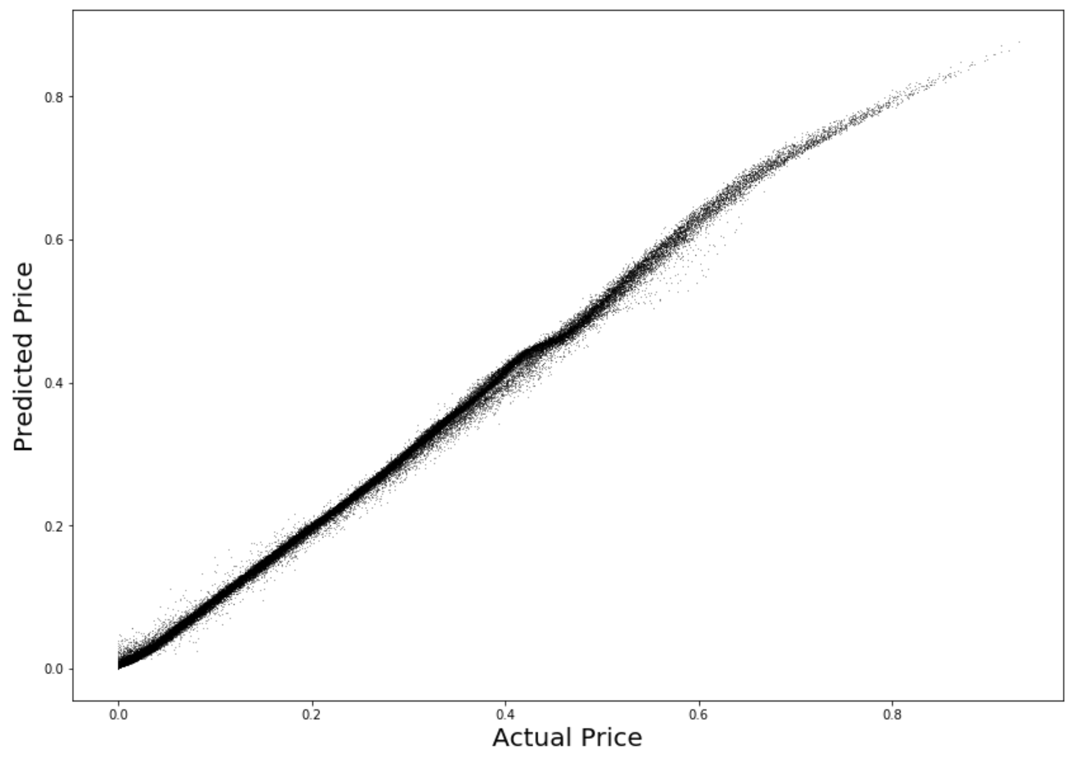
Figure 11.7: Out-of-sample data: Actual vs predicted prices

References

Culkin, Robert, and Sanjiv R. Das. 2017. “Machine Learning in Finance: The Case of Deep Learning for Option Pricing.” Journal of Investment Management 15 (4): 1–9.

Black, Fischer, and Myron Scholes. 1973. “The Pricing of Options and Corporate Liabilities.” Journal of Political Economy 81 (3): 637–54. https://EconPapers.repec.org/RePEc:ucp:jpolec:v:81:y:1973:i:3:p:637-54.