Chapter 6 Bayes Models: Learning from Experience
For a fairly good introduction to Bayes Rule, see Wikipedia, http://en.wikipedia.org/wiki/Bayes_theorem. The various R packages for Bayesian inference are at: http://cran.r-project.org/web/views/Bayesian.html.
In business, we often want to ask, is a given phenomena real or just a coincidence? Bayes theorem really helps with that. For example, we may ask – is Warren Buffet’s investment success a coincidence? How would you answer this question? Would it depend on your prior probability of Buffet being able to beat the market? How would this answer change as additional information about his performance was being released over time?
6.1 Bayes’ Theorem
Bayes rule follows easily from a decomposition of joint probability, i.e.,
\[ Pr[A \cap B] = Pr(A|B)\; Pr(B) = Pr(B|A)\; Pr(A) \]
Then the last two terms may be arranged to give
\[ Pr(A|B) = \frac{Pr(B|A)\; Pr(A)}{Pr(B)} \]
or
\[ Pr(B|A) = \frac{Pr(A|B)\; Pr(B)}{Pr(A)} \]
6.2 Example: Aids Testing
This is an interesting problem, because it shows that if you are diagnosed with AIDS, there is a good chance the diagnosis is wrong, but if you are diagnosed as not having AIDS then there is a good chance it is right - hopefully this is comforting news.
Define, \(\{Pos,Neg\}\) as a positive or negative diagnosis of having AIDS. Also define \(\{Dis, NoDis\}\) as the event of having the disease versus not having it. There are 1.5 million AIDS cases in the U.S. and about 300 million people which means the probability of AIDS in the population is 0.005 (half a percent). Hence, a random test will uncover someone with AIDS with a half a percent probability. The confirmation accuracy of the AIDS test is 99%, such that we have
\[ Pr(Pos | Dis) = 0.99 \]
Hence the test is reasonably good. The accuracy of the test for people who do not have AIDS is
\[ Pr(Neg | NoDis) = 0.95 \]
What we really want is the probability of having the disease when the test comes up positive, i.e. we need to compute \(Pr(Dis | Pos)\). Using Bayes Rule we calculate:
\[ \begin{aligned} Pr(Dis | Pos) &= \frac{Pr(Pos | Dis)Pr(Dis)}{Pr(Pos)} \\ &= \frac{Pr(Pos | Dis)Pr(Dis)}{Pr(Pos | Dis)Pr(Dis) + Pr(Pos|NoDis) Pr(NoDis)} \\ &= \frac{0.99 \times 0.005}{(0.99)(0.005) + (0.05)(0.995)} \\ &= 0.0904936 \end{aligned} \]
Hence, the chance of having AIDS when the test is positive is only 9%. We might also care about the chance of not having AIDS when the test is positive
\[ Pr(NoDis | Pos) = 1 - Pr(Dis | Pos) = 1 - 0.09 = 0.91 \]
Finally, what is the chance that we have AIDS even when the test is negative - this would also be a matter of concern to many of us, who might not relish the chance to be on some heavy drugs for the rest of our lives.
\[ \begin{aligned} Pr(Dis | Neg) &= \frac{Pr(Neg | Dis)Pr(Dis)}{Pr(Neg)} \\ &= \frac{Pr(Neg | Dis)Pr(Dis)}{Pr(Neg | Dis)Pr(Dis) + Pr(Neg|NoDis) Pr(NoDis)} \\ &= \frac{0.01 \times 0.005}{(0.01)(0.005) + (0.95)(0.995)} \\ &= 0.000053 \end{aligned} \]
Hence, this is a worry we should not have. If the test is negative, there is a miniscule chance that we are infected with AIDS.
6.3 Computational Approach using Sets
The preceding analysis is a good lead in to (a) the connection with joint probability distributions, and (b) using R to demonstrate a computational way of thinking about Bayes theorem.
Let’s begin by assuming that we have 300,000 people in the population, to scale down the numbers from the millions for convenience. Of these 1,500 have AIDS. So let’s create the population and then sample from it. See the use of the sample function in R.
#PEOPLE WITH AIDS
people = seq(1,300000)
people_aids = sample(people,1500)
people_noaids = setdiff(people,people_aids)
Note, how we also used the setdiff function to get the complement set of the people who do not have AIDS. Now, of the people who have AIDS, we know that 99% of them test positive so let’s subset that list, and also take its complement. These are joint events, and their numbers proscribe the joint distribution.
people_aids_pos = sample(people_aids,1500*0.99)
people_aids_neg = setdiff(people_aids,people_aids_pos)
print(length(people_aids_pos))
## [1] 1485print(length(people_aids_neg))## [1] 15people_aids_neg## [1] 35037 126781 139889 193826 149185 135464 28387 14428 257567 114212
## [11] 57248 151006 283192 168069 153407We can also subset the group that does not have AIDS, as we know that the test is negative for them 95% of the time.
#PEOPLE WITHOUT AIDS
people_noaids_neg = sample(people_noaids,298500*0.95)
people_noaids_pos = setdiff(people_noaids,people_noaids_neg)
print(length(people_noaids_neg))
## [1] 283575print(length(people_noaids_pos))## [1] 14925We can now compute the probability that someone actually has AIDS when the test comes out positive.
#HAVE AIDS GIVEN TEST IS POSITIVE
pr_aids_given_pos = (length(people_aids_pos))/
       (length(people_aids_pos)+length(people_noaids_pos))
pr_aids_given_pos
## [1] 0.0904936This confirms the formal Bayes computation that we had undertaken earlier. And of course, as we had examined earlier, what’s the chance that you have AIDS when the test is negative, i.e., a false negative?
#FALSE NEGATIVE: HAVE AIDS WHEN TEST IS NEGATIVE
pr_aids_given_neg = (length(people_aids_neg))/
       (length(people_aids_neg)+length(people_noaids_neg))
pr_aids_given_neg
## [1] 5.289326e-05Phew!
Note here that we first computed the joint sets covering joint outcomes, and then used these to compute conditional (Bayes) probabilities. The approach used R to apply a set-theoretic, computational approach to calculating conditional probabilities.
6.4 A Second Opinion
What if we tested positive, and then decided to get a second opinion, i.e., take another test. What would now be the posterior probability in this case? Here is the calculation.
#SECOND OPINION MEDICAL TEST FOR AIDS
0.99*0.09/(0.99*0.09 + 0.05*0.91)
## [1] 0.6619614Note that we used the previous posterior probability (0.91) as the prior probability in this calculation.
6.6 Continuous Space Bayes Theorem
In Bayesian approaches, the terms “prior”, “posterior”, and “likelihood” are commonly used and we explore this terminology here. We are usually interested in the parameter \(\theta\), the mean of the distribution of some data \(x\) (I am using the standard notation here). But in the Bayesian setting we do not just want the value of \(\theta\), but we want a distribution of values of \(\theta\) starting from some prior assumption about this distribution. So we start with \(p(\theta)\), which we call the prior distribution. We then observe data \(x\), and combine the data with the prior to get the posterior distribution \(p(\theta | x)\). To do this, we need to compute the probability of seeing the data \(x\) given our prior \(p(\theta)\) and this probability is given by the likelihood function \(L(x | \theta)\). Assume that the variance of the data \(x\) is known, i.e., is \(\sigma^2\).
6.6.1 Formulation
Applying Bayes’ theorem we have
\[ p(\theta | x) = \frac{L(x | \theta)\; p(\theta)}{\int L(x | \theta) \; p(\theta)\; d\theta} \propto L(x | \theta)\; p(\theta) \]
If we assume the prior distribution for the mean of the data is normal, i.e., \(p(\theta) \sim N[\mu_0, \sigma_0^2]\), and the likelihood is also normal, i.e., \(L(x | \theta) \sim N[\theta, \sigma^2]\), then we have that
\[ \begin{aligned} p(\theta) &= \frac{1}{\sqrt{2\pi \sigma_0^2}} \exp\left[-\frac{1}{2} \frac{(\theta-\mu_0)^2}{\sigma_0^2} \right] \sim N[\theta | \mu_0, \sigma_0^2] \; \; \propto \exp\left[-\frac{1}{2} \frac{(\theta-\mu_0)^2}{\sigma_0^2} \right] \\ L(x | \theta) &= \frac{1}{\sqrt{2\pi \sigma^2}} \exp\left[-\frac{1}{2} \frac{(x-\theta)^2}{\sigma^2} \right] \sim N[x | \theta, \sigma^2] \; \; \propto \exp\left[-\frac{1}{2} \frac{(x-\theta)^2}{\sigma^2} \right] \end{aligned} \]
6.6.2 Posterior Distribution
Given this, the posterior is as follows:
\[ p(\theta | x) \propto L(x | \theta) p(\theta) \;\; \propto \exp\left[-\frac{1}{2} \frac{(x-\theta)^2}{\sigma^2} -\frac{1}{2} \frac{(\theta-\mu_0)^2}{\sigma_0^2} \right] \]
Define the precision values to be \(\tau_0 = \frac{1}{\sigma_0^2}\), and \(\tau = \frac{1}{\sigma^2}\). Then it can be shown that when you observe a new value of the data \(x\), the posterior distribution is written down in closed form as:
\[ p(\theta | x) \sim N\left[ \frac{\tau_0}{\tau_0+\tau} \mu_0 + \frac{\tau}{\tau_0+\tau} x, \; \; \frac{1}{\tau_0 + \tau} \right] \]
When the posterior distribution and prior distribution have the same form, they are said to be “conjugate” with respect to the specific likelihood function.
6.6.3 Example
To take an example, suppose our prior for the mean of the equity premium per month is \(p(\theta) \sim N[0.005, 0.001^2]\). The standard deviation of the equity premium is 0.04. If next month we observe an equity premium of 1%, what is the posterior distribution of the mean equity premium?
mu0 = 0.005
sigma0 = 0.001
sigma=0.04
x = 0.01
tau0 = 1/sigma0^2
tau = 1/sigma^2
posterior_mean = tau0*mu0/(tau0+tau) + tau*x/(tau0+tau)
print(posterior_mean)
## [1] 0.005003123posterior_var = 1/(tau0+tau)
print(sqrt(posterior_var))## [1] 0.0009996876Hence, we see that after updating the mean has increased mildly because the data came in higher than expected.
6.6.4 General Formula for \(n\) sequential updates
If we observe \(n\) new values of \(x\), then the new posterior is
\[ p(\theta | x) \sim N\left[ \frac{\tau_0}{\tau_0+n\tau} \mu_0 + \frac{\tau}{\tau_0+n\tau} \sum_{j=1}^n x_j, \; \; \frac{1}{\tau_0 + n \tau} \right] \]
This is easy to derive, as it is just the result you obtain if you took each \(x_j\) and updated the posterior one at a time.
Try this as an Exercise. Estimate the equity risk premium. We will use data and discrete Bayes to come up with a forecast of the equity risk premium. Proceed along the following lines using the LearnBayes package.
- We’ll use data from 1926 onwards from the Fama-French data repository. All you need is the equity premium \((r_m-r_f)\) data, and I will leave it up to you to choose if you want to use annual or monthly data. Download this and load it into R.
- Using the series only up to the year 2000, present the descriptive statistics for the equity premium. State these in annualized terms.
- Present the distribution of returns as a histogram.
- Store the results of the histogram, i.e., the range of discrete values of the equity premium, and the probability of each one. Treat this as your prior distribution.
- Now take the remaining data for the years after 2000, and use this data to update the prior and construct a posterior. Assume that the prior, likelihood, and posterior are normally distributed. Use the discrete.bayes function to construct the posterior distribution and plot it using a histogram. See if you can put the prior and posterior on the same plot to see how the new data has changed the prior.
- What is the forecasted equity premium, and what is the confidence interval around your forecast?
6.7 Bayes Classifier
Suppose we want to classify entities (emails, consumers, companies, tumors, images, etc.) into categories \(c\). Think of a data set with rows each giving one instance of the data set with several characteristics, i.e., the \(x\) variables, and the row will also contain the category \(c\). Suppose there are \(n\) variables, and \(m\) categories.
We use the data to construct the prior and conditional probabilities. Once these probabilities are computed we say that the model is “trained”.
The trained classifier contains the unconditional probabilities \(p(c)\) of each class, which are merely frequencies with which each category appears. It also shows the conditional probability distributions \(p(x |c)\) given as the mean and standard deviation of the occurrence of these terms in each class.
The posterior probabilities are computed as follows. These tell us the most likely category given the data \(x\) on any observation.
\[ p(c=i | x_1,x_2,...,x_n) = \frac{p(x_1,x_2,...,x_n|c=i) \cdot p(c=i)}{\sum_{j=1}^m p(x_1,x_2,...,x_n|c=j) \cdot p(c=j)}, \quad \forall i=1,2,...,m \]
In the naive Bayes model, it is assumed that all the \(x\) variables are independent of each other, so that we may write
\[ p(x_1,x_2,...,x_n | c=i) = p(x_1 | c=i) \cdot p(x_1 | c=i) \cdot \cdot \cdot p(x_n | c=i) \]
We use the e1071 package. It has a one-line command that takes in the tagged training dataset using the function naiveBayes(). It returns the trained classifier model. We may take this trained model and re-apply to the training data set to see how well it does. We use the predict() function for this. The data set here is the classic Iris data.
6.7.1 Example
library(e1071)
data(iris)
print(head(iris))
## Sepal.Length Sepal.Width Petal.Length Petal.Width Species
## 1 5.1 3.5 1.4 0.2 setosa
## 2 4.9 3.0 1.4 0.2 setosa
## 3 4.7 3.2 1.3 0.2 setosa
## 4 4.6 3.1 1.5 0.2 setosa
## 5 5.0 3.6 1.4 0.2 setosa
## 6 5.4 3.9 1.7 0.4 setosatail(iris)## Sepal.Length Sepal.Width Petal.Length Petal.Width Species
## 145 6.7 3.3 5.7 2.5 virginica
## 146 6.7 3.0 5.2 2.3 virginica
## 147 6.3 2.5 5.0 1.9 virginica
## 148 6.5 3.0 5.2 2.0 virginica
## 149 6.2 3.4 5.4 2.3 virginica
## 150 5.9 3.0 5.1 1.8 virginica#NAIVE BAYES
res = naiveBayes(iris[,1:4],iris[,5])
#SHOWS THE PRIOR AND LIKELIHOOD FUNCTIONS
res##
## Naive Bayes Classifier for Discrete Predictors
##
## Call:
## naiveBayes.default(x = iris[, 1:4], y = iris[, 5])
##
## A-priori probabilities:
## iris[, 5]
## setosa versicolor virginica
## 0.3333333 0.3333333 0.3333333
##
## Conditional probabilities:
## Sepal.Length
## iris[, 5] [,1] [,2]
## setosa 5.006 0.3524897
## versicolor 5.936 0.5161711
## virginica 6.588 0.6358796
##
## Sepal.Width
## iris[, 5] [,1] [,2]
## setosa 3.428 0.3790644
## versicolor 2.770 0.3137983
## virginica 2.974 0.3224966
##
## Petal.Length
## iris[, 5] [,1] [,2]
## setosa 1.462 0.1736640
## versicolor 4.260 0.4699110
## virginica 5.552 0.5518947
##
## Petal.Width
## iris[, 5] [,1] [,2]
## setosa 0.246 0.1053856
## versicolor 1.326 0.1977527
## virginica 2.026 0.2746501#SHOWS POSTERIOR PROBABILITIES
predict(res,iris[,1:4],type="raw")## setosa versicolor virginica
## [1,] 1.000000e+00 2.981309e-18 2.152373e-25
## [2,] 1.000000e+00 3.169312e-17 6.938030e-25
## [3,] 1.000000e+00 2.367113e-18 7.240956e-26
## [4,] 1.000000e+00 3.069606e-17 8.690636e-25
## [5,] 1.000000e+00 1.017337e-18 8.885794e-26
## [6,] 1.000000e+00 2.717732e-14 4.344285e-21
## [7,] 1.000000e+00 2.321639e-17 7.988271e-25
## [8,] 1.000000e+00 1.390751e-17 8.166995e-25
## [9,] 1.000000e+00 1.990156e-17 3.606469e-25
## [10,] 1.000000e+00 7.378931e-18 3.615492e-25
## [11,] 1.000000e+00 9.396089e-18 1.474623e-24
## [12,] 1.000000e+00 3.461964e-17 2.093627e-24
## [13,] 1.000000e+00 2.804520e-18 1.010192e-25
## [14,] 1.000000e+00 1.799033e-19 6.060578e-27
## [15,] 1.000000e+00 5.533879e-19 2.485033e-25
## [16,] 1.000000e+00 6.273863e-17 4.509864e-23
## [17,] 1.000000e+00 1.106658e-16 1.282419e-23
## [18,] 1.000000e+00 4.841773e-17 2.350011e-24
## [19,] 1.000000e+00 1.126175e-14 2.567180e-21
## [20,] 1.000000e+00 1.808513e-17 1.963924e-24
## [21,] 1.000000e+00 2.178382e-15 2.013989e-22
## [22,] 1.000000e+00 1.210057e-15 7.788592e-23
## [23,] 1.000000e+00 4.535220e-20 3.130074e-27
## [24,] 1.000000e+00 3.147327e-11 8.175305e-19
## [25,] 1.000000e+00 1.838507e-14 1.553757e-21
## [26,] 1.000000e+00 6.873990e-16 1.830374e-23
## [27,] 1.000000e+00 3.192598e-14 1.045146e-21
## [28,] 1.000000e+00 1.542562e-17 1.274394e-24
## [29,] 1.000000e+00 8.833285e-18 5.368077e-25
## [30,] 1.000000e+00 9.557935e-17 3.652571e-24
## [31,] 1.000000e+00 2.166837e-16 6.730536e-24
## [32,] 1.000000e+00 3.940500e-14 1.546678e-21
## [33,] 1.000000e+00 1.609092e-20 1.013278e-26
## [34,] 1.000000e+00 7.222217e-20 4.261853e-26
## [35,] 1.000000e+00 6.289348e-17 1.831694e-24
## [36,] 1.000000e+00 2.850926e-18 8.874002e-26
## [37,] 1.000000e+00 7.746279e-18 7.235628e-25
## [38,] 1.000000e+00 8.623934e-20 1.223633e-26
## [39,] 1.000000e+00 4.612936e-18 9.655450e-26
## [40,] 1.000000e+00 2.009325e-17 1.237755e-24
## [41,] 1.000000e+00 1.300634e-17 5.657689e-25
## [42,] 1.000000e+00 1.577617e-15 5.717219e-24
## [43,] 1.000000e+00 1.494911e-18 4.800333e-26
## [44,] 1.000000e+00 1.076475e-10 3.721344e-18
## [45,] 1.000000e+00 1.357569e-12 1.708326e-19
## [46,] 1.000000e+00 3.882113e-16 5.587814e-24
## [47,] 1.000000e+00 5.086735e-18 8.960156e-25
## [48,] 1.000000e+00 5.012793e-18 1.636566e-25
## [49,] 1.000000e+00 5.717245e-18 8.231337e-25
## [50,] 1.000000e+00 7.713456e-18 3.349997e-25
## [51,] 4.893048e-107 8.018653e-01 1.981347e-01
## [52,] 7.920550e-100 9.429283e-01 5.707168e-02
## [53,] 5.494369e-121 4.606254e-01 5.393746e-01
## [54,] 1.129435e-69 9.999621e-01 3.789964e-05
## [55,] 1.473329e-105 9.503408e-01 4.965916e-02
## [56,] 1.931184e-89 9.990013e-01 9.986538e-04
## [57,] 4.539099e-113 6.592515e-01 3.407485e-01
## [58,] 2.549753e-34 9.999997e-01 3.119517e-07
## [59,] 6.562814e-97 9.895385e-01 1.046153e-02
## [60,] 5.000210e-69 9.998928e-01 1.071638e-04
## [61,] 7.354548e-41 9.999997e-01 3.143915e-07
## [62,] 4.799134e-86 9.958564e-01 4.143617e-03
## [63,] 4.631287e-60 9.999925e-01 7.541274e-06
## [64,] 1.052252e-103 9.850868e-01 1.491324e-02
## [65,] 4.789799e-55 9.999700e-01 2.999393e-05
## [66,] 1.514706e-92 9.787587e-01 2.124125e-02
## [67,] 1.338348e-97 9.899311e-01 1.006893e-02
## [68,] 2.026115e-62 9.999799e-01 2.007314e-05
## [69,] 6.547473e-101 9.941996e-01 5.800427e-03
## [70,] 3.016276e-58 9.999913e-01 8.739959e-06
## [71,] 1.053341e-127 1.609361e-01 8.390639e-01
## [72,] 1.248202e-70 9.997743e-01 2.256698e-04
## [73,] 3.294753e-119 9.245812e-01 7.541876e-02
## [74,] 1.314175e-95 9.979398e-01 2.060233e-03
## [75,] 3.003117e-83 9.982736e-01 1.726437e-03
## [76,] 2.536747e-92 9.865372e-01 1.346281e-02
## [77,] 1.558909e-111 9.102260e-01 8.977398e-02
## [78,] 7.014282e-136 7.989607e-02 9.201039e-01
## [79,] 5.034528e-99 9.854957e-01 1.450433e-02
## [80,] 1.439052e-41 9.999984e-01 1.601574e-06
## [81,] 1.251567e-54 9.999955e-01 4.500139e-06
## [82,] 8.769539e-48 9.999983e-01 1.742560e-06
## [83,] 3.447181e-62 9.999664e-01 3.361987e-05
## [84,] 1.087302e-132 6.134355e-01 3.865645e-01
## [85,] 4.119852e-97 9.918297e-01 8.170260e-03
## [86,] 1.140835e-102 8.734107e-01 1.265893e-01
## [87,] 2.247339e-110 7.971795e-01 2.028205e-01
## [88,] 4.870630e-88 9.992978e-01 7.022084e-04
## [89,] 2.028672e-72 9.997620e-01 2.379898e-04
## [90,] 2.227900e-69 9.999461e-01 5.390514e-05
## [91,] 5.110709e-81 9.998510e-01 1.489819e-04
## [92,] 5.774841e-99 9.885399e-01 1.146006e-02
## [93,] 5.146736e-66 9.999591e-01 4.089540e-05
## [94,] 1.332816e-34 9.999997e-01 2.716264e-07
## [95,] 6.094144e-77 9.998034e-01 1.966331e-04
## [96,] 1.424276e-72 9.998236e-01 1.764463e-04
## [97,] 8.302641e-77 9.996692e-01 3.307548e-04
## [98,] 1.835520e-82 9.988601e-01 1.139915e-03
## [99,] 5.710350e-30 9.999997e-01 3.094739e-07
## [100,] 3.996459e-73 9.998204e-01 1.795726e-04
## [101,] 3.993755e-249 1.031032e-10 1.000000e+00
## [102,] 1.228659e-149 2.724406e-02 9.727559e-01
## [103,] 2.460661e-216 2.327488e-07 9.999998e-01
## [104,] 2.864831e-173 2.290954e-03 9.977090e-01
## [105,] 8.299884e-214 3.175384e-07 9.999997e-01
## [106,] 1.371182e-267 3.807455e-10 1.000000e+00
## [107,] 3.444090e-107 9.719885e-01 2.801154e-02
## [108,] 3.741929e-224 1.782047e-06 9.999982e-01
## [109,] 5.564644e-188 5.823191e-04 9.994177e-01
## [110,] 2.052443e-260 2.461662e-12 1.000000e+00
## [111,] 8.669405e-159 4.895235e-04 9.995105e-01
## [112,] 4.220200e-163 3.168643e-03 9.968314e-01
## [113,] 4.360059e-190 6.230821e-06 9.999938e-01
## [114,] 6.142256e-151 1.423414e-02 9.857659e-01
## [115,] 2.201426e-186 1.393247e-06 9.999986e-01
## [116,] 2.949945e-191 6.128385e-07 9.999994e-01
## [117,] 2.909076e-168 2.152843e-03 9.978472e-01
## [118,] 1.347608e-281 2.872996e-12 1.000000e+00
## [119,] 2.786402e-306 1.151469e-12 1.000000e+00
## [120,] 2.082510e-123 9.561626e-01 4.383739e-02
## [121,] 2.194169e-217 1.712166e-08 1.000000e+00
## [122,] 3.325791e-145 1.518718e-02 9.848128e-01
## [123,] 6.251357e-269 1.170872e-09 1.000000e+00
## [124,] 4.415135e-135 1.360432e-01 8.639568e-01
## [125,] 6.315716e-201 1.300512e-06 9.999987e-01
## [126,] 5.257347e-203 9.507989e-06 9.999905e-01
## [127,] 1.476391e-129 2.067703e-01 7.932297e-01
## [128,] 8.772841e-134 1.130589e-01 8.869411e-01
## [129,] 5.230800e-194 1.395719e-05 9.999860e-01
## [130,] 7.014892e-179 8.232518e-04 9.991767e-01
## [131,] 6.306820e-218 1.214497e-06 9.999988e-01
## [132,] 2.539020e-247 4.668891e-10 1.000000e+00
## [133,] 2.210812e-201 2.000316e-06 9.999980e-01
## [134,] 1.128613e-128 7.118948e-01 2.881052e-01
## [135,] 8.114869e-151 4.900992e-01 5.099008e-01
## [136,] 7.419068e-249 1.448050e-10 1.000000e+00
## [137,] 1.004503e-215 9.743357e-09 1.000000e+00
## [138,] 1.346716e-167 2.186989e-03 9.978130e-01
## [139,] 1.994716e-128 1.999894e-01 8.000106e-01
## [140,] 8.440466e-185 6.769126e-06 9.999932e-01
## [141,] 2.334365e-218 7.456220e-09 1.000000e+00
## [142,] 2.179139e-183 6.352663e-07 9.999994e-01
## [143,] 1.228659e-149 2.724406e-02 9.727559e-01
## [144,] 3.426814e-229 6.597015e-09 1.000000e+00
## [145,] 2.011574e-232 2.620636e-10 1.000000e+00
## [146,] 1.078519e-187 7.915543e-07 9.999992e-01
## [147,] 1.061392e-146 2.770575e-02 9.722942e-01
## [148,] 1.846900e-164 4.398402e-04 9.995602e-01
## [149,] 1.439996e-195 3.384156e-07 9.999997e-01
## [150,] 2.771480e-143 5.987903e-02 9.401210e-01#CONFUSION MATRIX
out = table(predict(res,iris[,1:4]),iris[,5])
out##
## setosa versicolor virginica
## setosa 50 0 0
## versicolor 0 47 3
## virginica 0 3 476.8 Bayes Nets
Higher-dimension Bayes problems and joint distributions over several outcomes/events are easy to visualize with a network diagram, also called a Bayes net. A Bayes net is a directed, acyclic graph (known as a DAG), i.e., cycles are not permitted in the graph.
A good way to understand a Bayes net is with an example of economic distress. There are three levels at which distress may be noticed: economy level (\(E=1\)), industry level (\(I=1\)), or at a particular firm level (\(F=1\)). Economic distress can lead to industry distress and/or firm distress, and industry distress may or may not result in a firm’s distress.
The probabilities are as follows. Note that the probabilities in the first tableau are unconditional, but in all the subsequent tableaus they are conditional probabilities. See @(fig:bayesnet1).
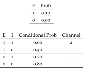
Figure 6.1: Conditional probabilities
The Bayes net shows the pathways of economic distress. There are three channels: \(a\) is the inducement of industry distress from economy distress; \(b\) is the inducement of firm distress directly from economy distress; \(c\) is the inducement of firm distress directly from industry distress. See @(fig:bayesnet2).
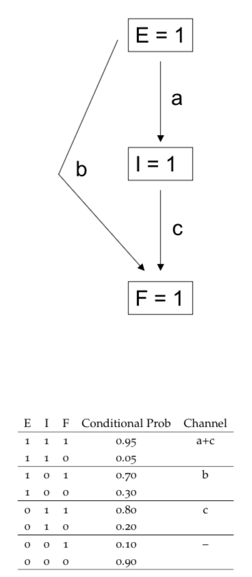
Figure 6.2: Bayesian network
Note here that each pair of conditional probabilities adds up to 1. The “channels” in the tableaus refer to the arrows in the Bayes net diagram.
6.8.0.1 Conditional Probability - 1
Now we will compute an answer to the question: What is the probability that the industry is distressed if the firm is known to be in distress? The calculation is as follows:
\[ \begin{aligned} Pr(I=1|F=1) &= \frac{Pr(F=1|I=1)\cdot Pr(I=1)}{Pr(F=1)} \\ Pr(F=1|I=1)\cdot Pr(I=1) &= Pr(F=1|I=1)\cdot Pr(I=1|E=1)\cdot Pr(E=1) \\ &+ Pr(F=1|I=1)\cdot Pr(I=1|E=0)\cdot Pr(E=0)\\ &= 0.95 \times 0.6 \times 0.1 + 0.8 \times 0.2 \times 0.9 = 0.201 \\ \end{aligned} \]
\[ \begin{aligned} Pr(F=1|I=0)\cdot Pr(I=0) &= Pr(F=1|I=0)\cdot Pr(I=0|E=1)\cdot Pr(E=1) \\ &+ Pr(F=1|I=0)\cdot Pr(I=0|E=0)\cdot Pr(E=0)\\ &= 0.7 \times 0.4 \times 0.1 + 0.1 \times 0.8 \times 0.9 = 0.100 \end{aligned} \]
\[ \begin{aligned} Pr(F=1) &= Pr(F=1|I=1)\cdot Pr(I=1) \\ &+ Pr(F=1|I=0)\cdot Pr(I=0) = 0.301 \end{aligned} \]
\[ Pr(I=1|F=1) = \frac{Pr(F=1|I=1)\cdot Pr(I=1)}{Pr(F=1)} = \frac{0.201}{0.301} = 0.6677741 \]
6.8.0.2 Computational set-theoretic approach
We may write a R script to compute the conditional probability that the industry is distressed when a firm is distressed. This uses the set approach that we visited earlier.
#BAYES NET COMPUTATIONS

E = seq(1,100000)
n = length(E)

E1 = sample(E,length(E)*0.1)
E0 = setdiff(E,E1)

E1I1 = sample(E1,length(E1)*0.6)
E1I0 = setdiff(E1,E1I1)
E0I1 = sample(E0,length(E0)*0.2)
E0I0 = setdiff(E0,E0I1)

E1I1F1 = sample(E1I1,length(E1I1)*0.95)
E1I1F0 = setdiff(E1I1,E1I1F1)
E1I0F1 = sample(E1I0,length(E1I0)*0.70)
E1I0F0 = setdiff(E1I0,E1I0F1)
E0I1F1 = sample(E0I1,length(E0I1)*0.80)
E0I1F0 = setdiff(E0I1,E0I1F1)
E0I0F1 = sample(E0I0,length(E0I0)*0.10)
E0I0F0 = setdiff(E0I0,E0I0F1)

pr_I1_given_F1 = length(c(E1I1F1,E0I1F1))/
     length(c(E1I1F1,E1I0F1,E0I1F1,E0I0F1))
print(pr_I1_given_F1)
## [1] 0.6677741Running this program gives the desired probability and confirms the previous result.
6.8.0.3 Conditional Probability - 2
Compute the conditional probability that the economy is in distress if the firm is in distress. Compare this to the previous conditional probability we computed of 0.6677741. Should it be lower?
pr_E1_given_F1 = length(c(E1I1F1,E1I0F1))/length(c(E1I1F1,E1I0F1,E0I1F1,E0I0F1))
print(pr_E1_given_F1)
## [1] 0.282392Yes, it should be lower than the probability that the industry is in distress when the firm is in distress, because the economy is one network layer removed from the firm, unlike the industry.
6.8.0.4 R Packages for Bayes Nets
What packages does R provide for doing Bayes Nets?
6.9 Bayes in Marketing
In pilot market tests (part of a larger market research campaign), Bayes theorem shows up in a simple manner. Suppose we have a project whose value is \(x\). If the product is successful (\(S\)), the payoff is \(+100\) and if the product fails (\(F\)) the payoff is \(-70\). The probability of these two events is:
\[ Pr(S) = 0.7, \quad Pr(F) = 0.3 \]
You can easily check that the expected value is \(E(x) = 49\). Suppose we were able to buy protection for a failed product, then this protection would be a put option (of the real option type), and would be worth \(0.3 \times 70 = 21\). Since the put saves the loss on failure, the value is simply the expected loss amount, conditional on loss. Market researchers think of this as the value of perfect information.
6.9.0.1 Product Launch?
Would you proceed with this product launch given these odds? Yes, the expected value is positive (note that we are assuming away risk aversion issues here - but this is not a finance topic, but a marketing research analysis).
6.9.0.2 Pilot Test
Now suppose there is an intermediate choice, i.e. you can undertake a pilot test (denoted \(T\)). Pilot tests are not highly accurate though they are reasonably sophisticated. The pilot test signals success (\(T+\)) or failure (\(T-\)) with the following probabilities:
\[ Pr(T+ | S) = 0.8 \\ Pr(T- | S) = 0.2 \\ Pr(T+ | F) = 0.3 \\ Pr(T- | F) = 0.7 \]
What are these? We note that \(Pr(T+ | S)\) stands for the probability that the pilot signals success when indeed the underlying product launch will be successful. Thus the pilot in this case gives only an accurate reading of success 80% of the time. Analogously, one can interpret the other probabilities.
We may compute the probability that the pilot gives a positive result:
\[ \begin{aligned} Pr(T+) &= Pr(T+ | S)Pr(S) + Pr(T+ | F)Pr(F) \\ &= (0.8)(0.7)+(0.3)(0.3) = 0.65 \end{aligned} \]
and that the result is negative:
\[ \begin{aligned} Pr(T-) &= Pr(T- | S)Pr(S) + Pr(T- | F)Pr(F) \\ &= (0.2)(0.7)+(0.7)(0.3) = 0.35 \end{aligned} \]
which now allows us to compute the following conditional probabilities:
\[ \begin{aligned} Pr(S | T+) &= \frac{Pr(T+|S)Pr(S)}{Pr(T+)} = \frac{(0.8)(0.7)}{0.65} = 0.86154 \\ Pr(S | T-) &= \frac{Pr(T-|S)Pr(S)}{Pr(T-)} = \frac{(0.2)(0.7)}{0.35} = 0.4 \\ Pr(F | T+) &= \frac{Pr(T+|F)Pr(F)}{Pr(T+)} = \frac{(0.3)(0.3)}{0.65} = 0.13846 \\ Pr(F | T-) &= \frac{Pr(T-|F)Pr(F)}{Pr(T-)} = \frac{(0.7)(0.3)}{0.35} = 0.6 \end{aligned} \]
Armed with these conditional probabilities, we may now re-evaluate our product launch. If the pilot comes out positive, what is the expected value of the product launch? This is as follows:
\[ E(x | T+) = 100 Pr(S|T+) +(-70) Pr(F|T+) \\ = 100(0.86154)-70(0.13846) \\ = 76.462 \]
And if the pilot comes out negative, then the value of the launch is:
\[ E(x | T-) = 100 Pr(S|T-) +(-70) Pr(F|T-) \\ = 100(0.4)-70(0.6) \\ = -2 \]
So. we see that if the pilot is negative, then we know that the expected value from the main product launch is negative, and we do not proceed. Thus, the overall expected value after the pilot is
\[ E(x) = E(x|T+)Pr(T+) + E(x|T-)Pr(T-) \\ = 76.462(0.65) + (0)(0.35) \\ = 49.70 \]
The incremental value over the case without the pilot test is \(0.70\). This is the information value of the pilot test.
6.10 Other Marketing Applications
Bayesian methods show up in many areas in the Marketing field. Especially around customer heterogeneity, see Allenby and Rossi (1998). Other papers are as follows:
- See the paper “The HB Revolution: How Bayesian Methods Have Changed the Face of Marketing Research,” by Allenby, Bakken, and Rossi (2004).
- See also the paper by David Bakken, titled ``The Bayesian Revolution in Marketing Research’’.
- In conjoint analysis, see the paper by Sawtooth software. https://www.sawtoothsoftware.com/download/techpap/undca15.pdf
References
Allenby, Greg M., and Peter Rossi. 1998. “Marketing Models of Consumer Heterogeneity.” Journal of Econometrics 89 (1-2): 57–78. http://EconPapers.repec.org/RePEc:eee:econom:v:89:y:1998:i:1-2:p:57-78.
Allenby, Greg M., David G. Bakken, and Peter E. Rossi. 2004. “The Hb Revolution: How Bayesian Methods Have Changed the Face of Marketing Research.” Marketing Research 16 (2): 20–25.