Chapter 7 More than Words: Text Analytics
7.1 Introduction
Text expands the universe of data many-fold. See my monograph on text mining in finance at: http://srdas.github.io/Das_TextAnalyticsInFinance.pdf
In Finance, for example, text has become a major source of trading information, leading to a new field known as News Metrics.
News analysis is defined as “the measurement of the various qualitative and quantitative attributes of textual news stories. Some of these attributes are: sentiment, relevance, and novelty. Expressing news stories as numbers permits the manipulation of everyday information in a mathematical and statistical way.” (Wikipedia). In this chapter, I provide a framework for text analytics techniques that are in widespread use. I will discuss various text analytic methods and software, and then provide a set of metrics that may be used to assess the performance of analytics. Various directions for this field are discussed through the exposition. The techniques herein can aid in the valuation and trading of securities, facilitate investment decision making, meet regulatory requirements, provide marketing insights, or manage risk.
“News analytics are used in financial modeling, particularly in quantitative and algorithmic trading. Further, news analytics can be used to plot and characterize firm behaviors over time and thus yield important strategic insights about rival firms. News analytics are usually derived through automated text analysis and applied to digital texts using elements from natural language processing and machine learning such as latent semantic analysis, support vector machines, `bag of words’, among other techniques.” (Wikipedia)
7.2 Text as Data
There are many reasons why text has business value. But this is a narrow view. Textual data provides a means of understanding all human behavior through a data-driven, analytical approach. Let’s enumerate some reasons for this.
- Big Text: there is more textual data than numerical data.
- Text is versatile. Nuances and behavioral expressions are not conveyed with numbers, so analyzing text allows us to explore these aspects of human interaction.
- Text contains emotive content. This has led to the ubiquity of “Sentiment analysis”. See for example: Admati-Pfleiderer 2001; DeMarzo et al 2003; Antweiler-Frank 2004, 2005; Das-Chen 2007; Tetlock 2007; Tetlock et al 2008; Mitra et al 2008; Leinweber-Sisk 2010.
- Text contains opinions and connections. See: Das et al 2005; Das and Sisk 2005; Godes et al 2005; Li 2006; Hochberg et al 2007.
- Numbers aggregate; text disaggregates. Text allows us to drill down into underlying behavior when understanding human interaction.
In a talk at the 17th ACM Conference on Information Knowledge and Management (CIKM ’08), Google’s director of research Peter Norvig stated his unequivocal preference for data over algorithms—“data is more agile than code.” Yet, it is well-understood that too much data can lead to overfitting so that an algorithm becomes mostly useless out-of-sample. 2. Chris Anderson: “Data is the New Theory.” 3. These issues are relevant to text mining, but let’s put them on hold till the end of the session.
7.3 Definition: Text-Mining
I will make an attempt to provide a comprehensive definition of “Text Mining”. As definitions go, it is often easier to enumerate various versions and nuances of an activity than to describe something in one single statement. So here goes:
- Text mining is the large-scale, automated processing of plain text language in digital form to extract data that is converted into useful quantitative or qualitative information.
- Text mining is automated on big data that is not amenable to human processing within reasonable time frames. It entails extracting data that is converted into information of many types.
- Simple: Text mining may be simple as key word searches and counts.
- Complicated: It may require language parsing and complex rules for information extraction.
- Involves structured text, such as the information in forms and some kinds of web pages.
- May be applied to unstructured text is a much harder endeavor.
- Text mining is also aimed at unearthing unseen relationships in unstructured text as in meta analyses of research papers, see Van Noorden 2012.
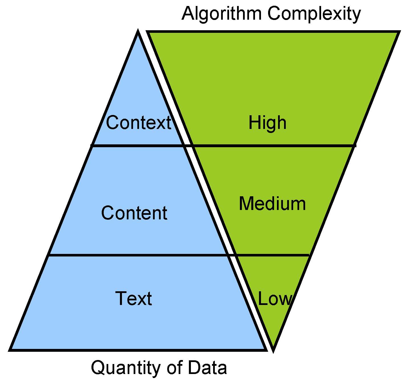
7.4 Data and Algorithms
7.5 Text Extraction
The R programming language is increasingly being used to download text from the web and then analyze it. The ease with which R may be used to scrape text from web site may be seen from the following simple command in R:
text = readLines("http://srdas.github.io/bio-candid.html")
text[15:20]
## [1] "journals. Prior to being an academic, he worked in the derivatives"
## [2] "business in the Asia-Pacific region as a Vice-President at"
## [3] "Citibank. His current research interests include: machine learning,"
## [4] "social networks, derivatives pricing models, portfolio theory, the"
## [5] "modeling of default risk, and venture capital. He has published over"
## [6] "ninety articles in academic journals, and has won numerous awards for"Here, we downloaded the my bio page from my university’s web site. It’s a simple HTML file.
length(text)## [1] 807.6 String Parsing
Suppose we just want the 17th line, we do:
text[17]## [1] "Citibank. His current research interests include: machine learning,"And, to find out the character length of the this line we use the function:
library(stringr)
str_length(text[17])
## [1] 67We have first invoked the library stringr that contains many string handling functions. In fact, we may also get the length of each line in the text vector by applying the function length() to the entire text vector.
text_len = str_length(text)
print(text_len)
## [1] 6 69 0 66 70 70 70 63 69 65 59 59 70 67 66 58 67 66 69 69 67 62 63
## [24] 19 0 0 56 0 65 67 66 65 64 66 69 63 69 65 27 0 3 0 71 71 69 68
## [47] 71 12 0 3 0 71 70 68 71 69 63 67 69 64 67 7 0 3 0 67 71 65 63
## [70] 72 69 68 66 69 70 70 43 0 0 0print(text_len[55])## [1] 71text_len[17]## [1] 677.7 Sort by Length
Some lines are very long and are the ones we are mainly interested in as they contain the bulk of the story, whereas many of the remaining lines that are shorter contain html formatting instructions. Thus, we may extract the top three lengthy lines with the following set of commands.
res = sort(text_len,decreasing=TRUE,index.return=TRUE)
idx = res$ix
text2 = text[idx]
text2
## [1] "important to open the academic door to the ivory tower and let the world"
## [2] "Sanjiv is now a Professor of Finance at Santa Clara University. He came"
## [3] "to SCU from Harvard Business School and spent a year at UC Berkeley. In"
## [4] "previous lives into his current existence, which is incredibly confused"
## [5] "Sanjiv's research style is instilled with a distinct \"New York state of"
## [6] "funds, the internet, portfolio choice, banking models, credit risk, and"
## [7] "ocean. The many walks in Greenwich village convinced him that there is"
## [8] "Santa Clara University's Leavey School of Business. He previously held"
## [9] "faculty appointments as Associate Professor at Harvard Business School"
## [10] "and UC Berkeley. He holds post-graduate degrees in Finance (M.Phil and"
## [11] "Management, co-editor of The Journal of Derivatives and The Journal of"
## [12] "mind\" - it is chaotic, diverse, with minimal method to the madness. He"
## [13] "any time you like, but you can never leave.\" Which is why he is doomed"
## [14] "to a lifetime in Hotel California. And he believes that, if this is as"
## [15] "<BODY background=\"http://algo.scu.edu/~sanjivdas/graphics/back2.gif\">"
## [16] "Berkeley), an MBA from the Indian Institute of Management, Ahmedabad,"
## [17] "modeling of default risk, and venture capital. He has published over"
## [18] "ninety articles in academic journals, and has won numerous awards for"
## [19] "science fiction movies, and writing cool software code. When there is"
## [20] "academic papers, which helps him relax. Always the contrarian, Sanjiv"
## [21] "his past life in the unreal world, Sanjiv worked at Citibank, N.A. in"
## [22] "has unpublished articles in many other areas. Some years ago, he took"
## [23] "There he learnt about the fascinating field of Randomized Algorithms,"
## [24] "in. Academia is a real challenge, given that he has to reconcile many"
## [25] "explains, you never really finish your education - \"you can check out"
## [26] "the Asia-Pacific region. He takes great pleasure in merging his many"
## [27] "has published articles on derivatives, term-structure models, mutual"
## [28] "more opinions than ideas. He has been known to have turned down many"
## [29] "Financial Services Research, and Associate Editor of other academic"
## [30] "Citibank. His current research interests include: machine learning,"
## [31] "research and teaching. His recent book \"Derivatives: Principles and"
## [32] "growing up, Sanjiv moved to New York to change the world, hopefully"
## [33] "confirming that an unchecked hobby can quickly become an obsession."
## [34] "pursuits, many of which stem from being in the epicenter of Silicon"
## [35] "Coastal living did a lot to mold Sanjiv, who needs to live near the"
## [36] "Sanjiv Das is the William and Janice Terry Professor of Finance at"
## [37] "journals. Prior to being an academic, he worked in the derivatives"
## [38] "social networks, derivatives pricing models, portfolio theory, the"
## [39] "through research. He graduated in 1994 with a Ph.D. from NYU, and"
## [40] "mountains meet the sea, riding sport motorbikes, reading, gadgets,"
## [41] "offers from Mad magazine to publish his academic work. As he often"
## [42] "B.Com in Accounting and Economics (University of Bombay, Sydenham"
## [43] "After loafing and working in many parts of Asia, but never really"
## [44] "since then spent five years in Boston, and now lives in San Jose,"
## [45] "thinks that New York City is the most calming place in the world,"
## [46] "no such thing as a representative investor, yet added many unique"
## [47] "California. Sanjiv loves animals, places in the world where the"
## [48] "skills he now applies earnestly to his editorial work, and other"
## [49] "Ph.D. from New York University), Computer Science (M.S. from UC"
## [50] "currently also serves as a Senior Fellow at the FDIC Center for"
## [51] "time available from the excitement of daily life, Sanjiv writes"
## [52] "time off to get another degree in computer science at Berkeley,"
## [53] "features to his personal utility function. He learnt that it is"
## [54] "Practice\" was published in May 2010 (second edition 2016). He"
## [55] "College), and is also a qualified Cost and Works Accountant"
## [56] "(AICWA). He is a senior editor of The Journal of Investment"
## [57] "business in the Asia-Pacific region as a Vice-President at"
## [58] "<p> <B>Sanjiv Das: A Short Academic Life History</B> <p>"
## [59] "bad as it gets, life is really pretty good."
## [60] "after California of course."
## [61] "Financial Research."
## [62] "and diverse."
## [63] "Valley."
## [64] "<HTML>"
## [65] "<p>"
## [66] "<p>"
## [67] "<p>"
## [68] ""
## [69] ""
## [70] ""
## [71] ""
## [72] ""
## [73] ""
## [74] ""
## [75] ""
## [76] ""
## [77] ""
## [78] ""
## [79] ""
## [80] ""7.8 Text cleanup
In short, text extraction can be exceedingly simple, though getting clean text is not as easy an operation. Removing html tags and other unnecessary elements in the file is also a fairly simple operation. We undertake the following steps that use generalized regular expressions (i.e., grep) to eliminate html formatting characters.
This will generate one single paragraph of text, relatively clean of formatting characters. Such a text collection is also known as a “bag of words”.
text = paste(text,collapse="\n")
print(text)
## [1] "<HTML>\n<BODY background=\"http://algo.scu.edu/~sanjivdas/graphics/back2.gif\">\n\nSanjiv Das is the William and Janice Terry Professor of Finance at\nSanta Clara University's Leavey School of Business. He previously held\nfaculty appointments as Associate Professor at Harvard Business School\nand UC Berkeley. He holds post-graduate degrees in Finance (M.Phil and\nPh.D. from New York University), Computer Science (M.S. from UC\nBerkeley), an MBA from the Indian Institute of Management, Ahmedabad,\nB.Com in Accounting and Economics (University of Bombay, Sydenham\nCollege), and is also a qualified Cost and Works Accountant\n(AICWA). He is a senior editor of The Journal of Investment\nManagement, co-editor of The Journal of Derivatives and The Journal of\nFinancial Services Research, and Associate Editor of other academic\njournals. Prior to being an academic, he worked in the derivatives\nbusiness in the Asia-Pacific region as a Vice-President at\nCitibank. His current research interests include: machine learning,\nsocial networks, derivatives pricing models, portfolio theory, the\nmodeling of default risk, and venture capital. He has published over\nninety articles in academic journals, and has won numerous awards for\nresearch and teaching. His recent book \"Derivatives: Principles and\nPractice\" was published in May 2010 (second edition 2016). He\ncurrently also serves as a Senior Fellow at the FDIC Center for\nFinancial Research.\n\n\n<p> <B>Sanjiv Das: A Short Academic Life History</B> <p>\n\nAfter loafing and working in many parts of Asia, but never really\ngrowing up, Sanjiv moved to New York to change the world, hopefully\nthrough research. He graduated in 1994 with a Ph.D. from NYU, and\nsince then spent five years in Boston, and now lives in San Jose,\nCalifornia. Sanjiv loves animals, places in the world where the\nmountains meet the sea, riding sport motorbikes, reading, gadgets,\nscience fiction movies, and writing cool software code. When there is\ntime available from the excitement of daily life, Sanjiv writes\nacademic papers, which helps him relax. Always the contrarian, Sanjiv\nthinks that New York City is the most calming place in the world,\nafter California of course.\n\n<p>\n\nSanjiv is now a Professor of Finance at Santa Clara University. He came\nto SCU from Harvard Business School and spent a year at UC Berkeley. In\nhis past life in the unreal world, Sanjiv worked at Citibank, N.A. in\nthe Asia-Pacific region. He takes great pleasure in merging his many\nprevious lives into his current existence, which is incredibly confused\nand diverse.\n\n<p>\n\nSanjiv's research style is instilled with a distinct \"New York state of\nmind\" - it is chaotic, diverse, with minimal method to the madness. He\nhas published articles on derivatives, term-structure models, mutual\nfunds, the internet, portfolio choice, banking models, credit risk, and\nhas unpublished articles in many other areas. Some years ago, he took\ntime off to get another degree in computer science at Berkeley,\nconfirming that an unchecked hobby can quickly become an obsession.\nThere he learnt about the fascinating field of Randomized Algorithms,\nskills he now applies earnestly to his editorial work, and other\npursuits, many of which stem from being in the epicenter of Silicon\nValley.\n\n<p>\n\nCoastal living did a lot to mold Sanjiv, who needs to live near the\nocean. The many walks in Greenwich village convinced him that there is\nno such thing as a representative investor, yet added many unique\nfeatures to his personal utility function. He learnt that it is\nimportant to open the academic door to the ivory tower and let the world\nin. Academia is a real challenge, given that he has to reconcile many\nmore opinions than ideas. He has been known to have turned down many\noffers from Mad magazine to publish his academic work. As he often\nexplains, you never really finish your education - \"you can check out\nany time you like, but you can never leave.\" Which is why he is doomed\nto a lifetime in Hotel California. And he believes that, if this is as\nbad as it gets, life is really pretty good.\n\n\n"text = str_replace_all(text,"[<>{}()&;,.\n]"," ")
print(text)## [1] " HTML BODY background=\"http://algo scu edu/~sanjivdas/graphics/back2 gif\" Sanjiv Das is the William and Janice Terry Professor of Finance at Santa Clara University's Leavey School of Business He previously held faculty appointments as Associate Professor at Harvard Business School and UC Berkeley He holds post-graduate degrees in Finance M Phil and Ph D from New York University Computer Science M S from UC Berkeley an MBA from the Indian Institute of Management Ahmedabad B Com in Accounting and Economics University of Bombay Sydenham College and is also a qualified Cost and Works Accountant AICWA He is a senior editor of The Journal of Investment Management co-editor of The Journal of Derivatives and The Journal of Financial Services Research and Associate Editor of other academic journals Prior to being an academic he worked in the derivatives business in the Asia-Pacific region as a Vice-President at Citibank His current research interests include: machine learning social networks derivatives pricing models portfolio theory the modeling of default risk and venture capital He has published over ninety articles in academic journals and has won numerous awards for research and teaching His recent book \"Derivatives: Principles and Practice\" was published in May 2010 second edition 2016 He currently also serves as a Senior Fellow at the FDIC Center for Financial Research p B Sanjiv Das: A Short Academic Life History /B p After loafing and working in many parts of Asia but never really growing up Sanjiv moved to New York to change the world hopefully through research He graduated in 1994 with a Ph D from NYU and since then spent five years in Boston and now lives in San Jose California Sanjiv loves animals places in the world where the mountains meet the sea riding sport motorbikes reading gadgets science fiction movies and writing cool software code When there is time available from the excitement of daily life Sanjiv writes academic papers which helps him relax Always the contrarian Sanjiv thinks that New York City is the most calming place in the world after California of course p Sanjiv is now a Professor of Finance at Santa Clara University He came to SCU from Harvard Business School and spent a year at UC Berkeley In his past life in the unreal world Sanjiv worked at Citibank N A in the Asia-Pacific region He takes great pleasure in merging his many previous lives into his current existence which is incredibly confused and diverse p Sanjiv's research style is instilled with a distinct \"New York state of mind\" - it is chaotic diverse with minimal method to the madness He has published articles on derivatives term-structure models mutual funds the internet portfolio choice banking models credit risk and has unpublished articles in many other areas Some years ago he took time off to get another degree in computer science at Berkeley confirming that an unchecked hobby can quickly become an obsession There he learnt about the fascinating field of Randomized Algorithms skills he now applies earnestly to his editorial work and other pursuits many of which stem from being in the epicenter of Silicon Valley p Coastal living did a lot to mold Sanjiv who needs to live near the ocean The many walks in Greenwich village convinced him that there is no such thing as a representative investor yet added many unique features to his personal utility function He learnt that it is important to open the academic door to the ivory tower and let the world in Academia is a real challenge given that he has to reconcile many more opinions than ideas He has been known to have turned down many offers from Mad magazine to publish his academic work As he often explains you never really finish your education - \"you can check out any time you like but you can never leave \" Which is why he is doomed to a lifetime in Hotel California And he believes that if this is as bad as it gets life is really pretty good "7.9 The XML Package
The XML package in R also comes with many functions that aid in cleaning up text and dropping it (mostly unformatted) into a flat file or data frame. This may then be further processed. Here is some example code for this.
7.9.1 Processing XML files in R into a data frame
The following example has been adapted from r-bloggers.com. It uses the following URL:
http://www.w3schools.com/xml/plant_catalog.xml
library(XML)
#Part1: Reading an xml and creating a data frame with it.

xml.url <- "http://www.w3schools.com/xml/plant_catalog.xml"
xmlfile <- xmlTreeParse(xml.url)
xmltop <- xmlRoot(xmlfile)
plantcat <- xmlSApply(xmltop, function(x) xmlSApply(x, xmlValue))
plantcat_df <- data.frame(t(plantcat),row.names=NULL)
plantcat_df[1:5,1:4]
7.9.2 Creating a XML file from a data frame
library(XML)## Warning: package 'XML' was built under R version 3.3.2## Loading required package: methods#Example adapted from https://stat.ethz.ch/pipermail/r-help/2008-September/175364.html
#Load the iris data set and create a data frame
data("iris")
data <- as.data.frame(iris)
xml <- xmlTree()
xml$addTag("document", close=FALSE)## Warning in xmlRoot.XMLInternalDocument(currentNodes[[1]]): empty XML
## documentfor (i in 1:nrow(data)) {
xml$addTag("row", close=FALSE)
for (j in names(data)) {
xml$addTag(j, data[i, j])
}
xml$closeTag()
}
xml$closeTag()
#view the xml (uncomment line below to see XML, long output)
cat(saveXML(xml))## <?xml version="1.0"?>
##
## <document>
## <row>
## <Sepal.Length>5.1</Sepal.Length>
## <Sepal.Width>3.5</Sepal.Width>
## <Petal.Length>1.4</Petal.Length>
## <Petal.Width>0.2</Petal.Width>
## <Species>setosa</Species>
## </row>
## <row>
## <Sepal.Length>4.9</Sepal.Length>
## <Sepal.Width>3</Sepal.Width>
## <Petal.Length>1.4</Petal.Length>
## <Petal.Width>0.2</Petal.Width>
## <Species>setosa</Species>
## </row>
## <row>
## <Sepal.Length>4.7</Sepal.Length>
## <Sepal.Width>3.2</Sepal.Width>
## <Petal.Length>1.3</Petal.Length>
## <Petal.Width>0.2</Petal.Width>
## <Species>setosa</Species>
## </row>
## <row>
## <Sepal.Length>4.6</Sepal.Length>
## <Sepal.Width>3.1</Sepal.Width>
## <Petal.Length>1.5</Petal.Length>
## <Petal.Width>0.2</Petal.Width>
## <Species>setosa</Species>
## </row>
## <row>
## <Sepal.Length>5</Sepal.Length>
## <Sepal.Width>3.6</Sepal.Width>
## <Petal.Length>1.4</Petal.Length>
## <Petal.Width>0.2</Petal.Width>
## <Species>setosa</Species>
## </row>
## <row>
## <Sepal.Length>5.4</Sepal.Length>
## <Sepal.Width>3.9</Sepal.Width>
## <Petal.Length>1.7</Petal.Length>
## <Petal.Width>0.4</Petal.Width>
## <Species>setosa</Species>
## </row>
## <row>
## <Sepal.Length>4.6</Sepal.Length>
## <Sepal.Width>3.4</Sepal.Width>
## <Petal.Length>1.4</Petal.Length>
## <Petal.Width>0.3</Petal.Width>
## <Species>setosa</Species>
## </row>
## <row>
## <Sepal.Length>5</Sepal.Length>
## <Sepal.Width>3.4</Sepal.Width>
## <Petal.Length>1.5</Petal.Length>
## <Petal.Width>0.2</Petal.Width>
## <Species>setosa</Species>
## </row>
## <row>
## <Sepal.Length>4.4</Sepal.Length>
## <Sepal.Width>2.9</Sepal.Width>
## <Petal.Length>1.4</Petal.Length>
## <Petal.Width>0.2</Petal.Width>
## <Species>setosa</Species>
## </row>
## <row>
## <Sepal.Length>4.9</Sepal.Length>
## <Sepal.Width>3.1</Sepal.Width>
## <Petal.Length>1.5</Petal.Length>
## <Petal.Width>0.1</Petal.Width>
## <Species>setosa</Species>
## </row>
## <row>
## <Sepal.Length>5.4</Sepal.Length>
## <Sepal.Width>3.7</Sepal.Width>
## <Petal.Length>1.5</Petal.Length>
## <Petal.Width>0.2</Petal.Width>
## <Species>setosa</Species>
## </row>
## <row>
## <Sepal.Length>4.8</Sepal.Length>
## <Sepal.Width>3.4</Sepal.Width>
## <Petal.Length>1.6</Petal.Length>
## <Petal.Width>0.2</Petal.Width>
## <Species>setosa</Species>
## </row>
## <row>
## <Sepal.Length>4.8</Sepal.Length>
## <Sepal.Width>3</Sepal.Width>
## <Petal.Length>1.4</Petal.Length>
## <Petal.Width>0.1</Petal.Width>
## <Species>setosa</Species>
## </row>
## <row>
## <Sepal.Length>4.3</Sepal.Length>
## <Sepal.Width>3</Sepal.Width>
## <Petal.Length>1.1</Petal.Length>
## <Petal.Width>0.1</Petal.Width>
## <Species>setosa</Species>
## </row>
## <row>
## <Sepal.Length>5.8</Sepal.Length>
## <Sepal.Width>4</Sepal.Width>
## <Petal.Length>1.2</Petal.Length>
## <Petal.Width>0.2</Petal.Width>
## <Species>setosa</Species>
## </row>
## <row>
## <Sepal.Length>5.7</Sepal.Length>
## <Sepal.Width>4.4</Sepal.Width>
## <Petal.Length>1.5</Petal.Length>
## <Petal.Width>0.4</Petal.Width>
## <Species>setosa</Species>
## </row>
## <row>
## <Sepal.Length>5.4</Sepal.Length>
## <Sepal.Width>3.9</Sepal.Width>
## <Petal.Length>1.3</Petal.Length>
## <Petal.Width>0.4</Petal.Width>
## <Species>setosa</Species>
## </row>
## <row>
## <Sepal.Length>5.1</Sepal.Length>
## <Sepal.Width>3.5</Sepal.Width>
## <Petal.Length>1.4</Petal.Length>
## <Petal.Width>0.3</Petal.Width>
## <Species>setosa</Species>
## </row>
## <row>
## <Sepal.Length>5.7</Sepal.Length>
## <Sepal.Width>3.8</Sepal.Width>
## <Petal.Length>1.7</Petal.Length>
## <Petal.Width>0.3</Petal.Width>
## <Species>setosa</Species>
## </row>
## <row>
## <Sepal.Length>5.1</Sepal.Length>
## <Sepal.Width>3.8</Sepal.Width>
## <Petal.Length>1.5</Petal.Length>
## <Petal.Width>0.3</Petal.Width>
## <Species>setosa</Species>
## </row>
## <row>
## <Sepal.Length>5.4</Sepal.Length>
## <Sepal.Width>3.4</Sepal.Width>
## <Petal.Length>1.7</Petal.Length>
## <Petal.Width>0.2</Petal.Width>
## <Species>setosa</Species>
## </row>
## <row>
## <Sepal.Length>5.1</Sepal.Length>
## <Sepal.Width>3.7</Sepal.Width>
## <Petal.Length>1.5</Petal.Length>
## <Petal.Width>0.4</Petal.Width>
## <Species>setosa</Species>
## </row>
## <row>
## <Sepal.Length>4.6</Sepal.Length>
## <Sepal.Width>3.6</Sepal.Width>
## <Petal.Length>1</Petal.Length>
## <Petal.Width>0.2</Petal.Width>
## <Species>setosa</Species>
## </row>
## <row>
## <Sepal.Length>5.1</Sepal.Length>
## <Sepal.Width>3.3</Sepal.Width>
## <Petal.Length>1.7</Petal.Length>
## <Petal.Width>0.5</Petal.Width>
## <Species>setosa</Species>
## </row>
## <row>
## <Sepal.Length>4.8</Sepal.Length>
## <Sepal.Width>3.4</Sepal.Width>
## <Petal.Length>1.9</Petal.Length>
## <Petal.Width>0.2</Petal.Width>
## <Species>setosa</Species>
## </row>
## <row>
## <Sepal.Length>5</Sepal.Length>
## <Sepal.Width>3</Sepal.Width>
## <Petal.Length>1.6</Petal.Length>
## <Petal.Width>0.2</Petal.Width>
## <Species>setosa</Species>
## </row>
## <row>
## <Sepal.Length>5</Sepal.Length>
## <Sepal.Width>3.4</Sepal.Width>
## <Petal.Length>1.6</Petal.Length>
## <Petal.Width>0.4</Petal.Width>
## <Species>setosa</Species>
## </row>
## <row>
## <Sepal.Length>5.2</Sepal.Length>
## <Sepal.Width>3.5</Sepal.Width>
## <Petal.Length>1.5</Petal.Length>
## <Petal.Width>0.2</Petal.Width>
## <Species>setosa</Species>
## </row>
## <row>
## <Sepal.Length>5.2</Sepal.Length>
## <Sepal.Width>3.4</Sepal.Width>
## <Petal.Length>1.4</Petal.Length>
## <Petal.Width>0.2</Petal.Width>
## <Species>setosa</Species>
## </row>
## <row>
## <Sepal.Length>4.7</Sepal.Length>
## <Sepal.Width>3.2</Sepal.Width>
## <Petal.Length>1.6</Petal.Length>
## <Petal.Width>0.2</Petal.Width>
## <Species>setosa</Species>
## </row>
## <row>
## <Sepal.Length>4.8</Sepal.Length>
## <Sepal.Width>3.1</Sepal.Width>
## <Petal.Length>1.6</Petal.Length>
## <Petal.Width>0.2</Petal.Width>
## <Species>setosa</Species>
## </row>
## <row>
## <Sepal.Length>5.4</Sepal.Length>
## <Sepal.Width>3.4</Sepal.Width>
## <Petal.Length>1.5</Petal.Length>
## <Petal.Width>0.4</Petal.Width>
## <Species>setosa</Species>
## </row>
## <row>
## <Sepal.Length>5.2</Sepal.Length>
## <Sepal.Width>4.1</Sepal.Width>
## <Petal.Length>1.5</Petal.Length>
## <Petal.Width>0.1</Petal.Width>
## <Species>setosa</Species>
## </row>
## <row>
## <Sepal.Length>5.5</Sepal.Length>
## <Sepal.Width>4.2</Sepal.Width>
## <Petal.Length>1.4</Petal.Length>
## <Petal.Width>0.2</Petal.Width>
## <Species>setosa</Species>
## </row>
## <row>
## <Sepal.Length>4.9</Sepal.Length>
## <Sepal.Width>3.1</Sepal.Width>
## <Petal.Length>1.5</Petal.Length>
## <Petal.Width>0.2</Petal.Width>
## <Species>setosa</Species>
## </row>
## <row>
## <Sepal.Length>5</Sepal.Length>
## <Sepal.Width>3.2</Sepal.Width>
## <Petal.Length>1.2</Petal.Length>
## <Petal.Width>0.2</Petal.Width>
## <Species>setosa</Species>
## </row>
## <row>
## <Sepal.Length>5.5</Sepal.Length>
## <Sepal.Width>3.5</Sepal.Width>
## <Petal.Length>1.3</Petal.Length>
## <Petal.Width>0.2</Petal.Width>
## <Species>setosa</Species>
## </row>
## <row>
## <Sepal.Length>4.9</Sepal.Length>
## <Sepal.Width>3.6</Sepal.Width>
## <Petal.Length>1.4</Petal.Length>
## <Petal.Width>0.1</Petal.Width>
## <Species>setosa</Species>
## </row>
## <row>
## <Sepal.Length>4.4</Sepal.Length>
## <Sepal.Width>3</Sepal.Width>
## <Petal.Length>1.3</Petal.Length>
## <Petal.Width>0.2</Petal.Width>
## <Species>setosa</Species>
## </row>
## <row>
## <Sepal.Length>5.1</Sepal.Length>
## <Sepal.Width>3.4</Sepal.Width>
## <Petal.Length>1.5</Petal.Length>
## <Petal.Width>0.2</Petal.Width>
## <Species>setosa</Species>
## </row>
## <row>
## <Sepal.Length>5</Sepal.Length>
## <Sepal.Width>3.5</Sepal.Width>
## <Petal.Length>1.3</Petal.Length>
## <Petal.Width>0.3</Petal.Width>
## <Species>setosa</Species>
## </row>
## <row>
## <Sepal.Length>4.5</Sepal.Length>
## <Sepal.Width>2.3</Sepal.Width>
## <Petal.Length>1.3</Petal.Length>
## <Petal.Width>0.3</Petal.Width>
## <Species>setosa</Species>
## </row>
## <row>
## <Sepal.Length>4.4</Sepal.Length>
## <Sepal.Width>3.2</Sepal.Width>
## <Petal.Length>1.3</Petal.Length>
## <Petal.Width>0.2</Petal.Width>
## <Species>setosa</Species>
## </row>
## <row>
## <Sepal.Length>5</Sepal.Length>
## <Sepal.Width>3.5</Sepal.Width>
## <Petal.Length>1.6</Petal.Length>
## <Petal.Width>0.6</Petal.Width>
## <Species>setosa</Species>
## </row>
## <row>
## <Sepal.Length>5.1</Sepal.Length>
## <Sepal.Width>3.8</Sepal.Width>
## <Petal.Length>1.9</Petal.Length>
## <Petal.Width>0.4</Petal.Width>
## <Species>setosa</Species>
## </row>
## <row>
## <Sepal.Length>4.8</Sepal.Length>
## <Sepal.Width>3</Sepal.Width>
## <Petal.Length>1.4</Petal.Length>
## <Petal.Width>0.3</Petal.Width>
## <Species>setosa</Species>
## </row>
## <row>
## <Sepal.Length>5.1</Sepal.Length>
## <Sepal.Width>3.8</Sepal.Width>
## <Petal.Length>1.6</Petal.Length>
## <Petal.Width>0.2</Petal.Width>
## <Species>setosa</Species>
## </row>
## <row>
## <Sepal.Length>4.6</Sepal.Length>
## <Sepal.Width>3.2</Sepal.Width>
## <Petal.Length>1.4</Petal.Length>
## <Petal.Width>0.2</Petal.Width>
## <Species>setosa</Species>
## </row>
## <row>
## <Sepal.Length>5.3</Sepal.Length>
## <Sepal.Width>3.7</Sepal.Width>
## <Petal.Length>1.5</Petal.Length>
## <Petal.Width>0.2</Petal.Width>
## <Species>setosa</Species>
## </row>
## <row>
## <Sepal.Length>5</Sepal.Length>
## <Sepal.Width>3.3</Sepal.Width>
## <Petal.Length>1.4</Petal.Length>
## <Petal.Width>0.2</Petal.Width>
## <Species>setosa</Species>
## </row>
## <row>
## <Sepal.Length>7</Sepal.Length>
## <Sepal.Width>3.2</Sepal.Width>
## <Petal.Length>4.7</Petal.Length>
## <Petal.Width>1.4</Petal.Width>
## <Species>versicolor</Species>
## </row>
## <row>
## <Sepal.Length>6.4</Sepal.Length>
## <Sepal.Width>3.2</Sepal.Width>
## <Petal.Length>4.5</Petal.Length>
## <Petal.Width>1.5</Petal.Width>
## <Species>versicolor</Species>
## </row>
## <row>
## <Sepal.Length>6.9</Sepal.Length>
## <Sepal.Width>3.1</Sepal.Width>
## <Petal.Length>4.9</Petal.Length>
## <Petal.Width>1.5</Petal.Width>
## <Species>versicolor</Species>
## </row>
## <row>
## <Sepal.Length>5.5</Sepal.Length>
## <Sepal.Width>2.3</Sepal.Width>
## <Petal.Length>4</Petal.Length>
## <Petal.Width>1.3</Petal.Width>
## <Species>versicolor</Species>
## </row>
## <row>
## <Sepal.Length>6.5</Sepal.Length>
## <Sepal.Width>2.8</Sepal.Width>
## <Petal.Length>4.6</Petal.Length>
## <Petal.Width>1.5</Petal.Width>
## <Species>versicolor</Species>
## </row>
## <row>
## <Sepal.Length>5.7</Sepal.Length>
## <Sepal.Width>2.8</Sepal.Width>
## <Petal.Length>4.5</Petal.Length>
## <Petal.Width>1.3</Petal.Width>
## <Species>versicolor</Species>
## </row>
## <row>
## <Sepal.Length>6.3</Sepal.Length>
## <Sepal.Width>3.3</Sepal.Width>
## <Petal.Length>4.7</Petal.Length>
## <Petal.Width>1.6</Petal.Width>
## <Species>versicolor</Species>
## </row>
## <row>
## <Sepal.Length>4.9</Sepal.Length>
## <Sepal.Width>2.4</Sepal.Width>
## <Petal.Length>3.3</Petal.Length>
## <Petal.Width>1</Petal.Width>
## <Species>versicolor</Species>
## </row>
## <row>
## <Sepal.Length>6.6</Sepal.Length>
## <Sepal.Width>2.9</Sepal.Width>
## <Petal.Length>4.6</Petal.Length>
## <Petal.Width>1.3</Petal.Width>
## <Species>versicolor</Species>
## </row>
## <row>
## <Sepal.Length>5.2</Sepal.Length>
## <Sepal.Width>2.7</Sepal.Width>
## <Petal.Length>3.9</Petal.Length>
## <Petal.Width>1.4</Petal.Width>
## <Species>versicolor</Species>
## </row>
## <row>
## <Sepal.Length>5</Sepal.Length>
## <Sepal.Width>2</Sepal.Width>
## <Petal.Length>3.5</Petal.Length>
## <Petal.Width>1</Petal.Width>
## <Species>versicolor</Species>
## </row>
## <row>
## <Sepal.Length>5.9</Sepal.Length>
## <Sepal.Width>3</Sepal.Width>
## <Petal.Length>4.2</Petal.Length>
## <Petal.Width>1.5</Petal.Width>
## <Species>versicolor</Species>
## </row>
## <row>
## <Sepal.Length>6</Sepal.Length>
## <Sepal.Width>2.2</Sepal.Width>
## <Petal.Length>4</Petal.Length>
## <Petal.Width>1</Petal.Width>
## <Species>versicolor</Species>
## </row>
## <row>
## <Sepal.Length>6.1</Sepal.Length>
## <Sepal.Width>2.9</Sepal.Width>
## <Petal.Length>4.7</Petal.Length>
## <Petal.Width>1.4</Petal.Width>
## <Species>versicolor</Species>
## </row>
## <row>
## <Sepal.Length>5.6</Sepal.Length>
## <Sepal.Width>2.9</Sepal.Width>
## <Petal.Length>3.6</Petal.Length>
## <Petal.Width>1.3</Petal.Width>
## <Species>versicolor</Species>
## </row>
## <row>
## <Sepal.Length>6.7</Sepal.Length>
## <Sepal.Width>3.1</Sepal.Width>
## <Petal.Length>4.4</Petal.Length>
## <Petal.Width>1.4</Petal.Width>
## <Species>versicolor</Species>
## </row>
## <row>
## <Sepal.Length>5.6</Sepal.Length>
## <Sepal.Width>3</Sepal.Width>
## <Petal.Length>4.5</Petal.Length>
## <Petal.Width>1.5</Petal.Width>
## <Species>versicolor</Species>
## </row>
## <row>
## <Sepal.Length>5.8</Sepal.Length>
## <Sepal.Width>2.7</Sepal.Width>
## <Petal.Length>4.1</Petal.Length>
## <Petal.Width>1</Petal.Width>
## <Species>versicolor</Species>
## </row>
## <row>
## <Sepal.Length>6.2</Sepal.Length>
## <Sepal.Width>2.2</Sepal.Width>
## <Petal.Length>4.5</Petal.Length>
## <Petal.Width>1.5</Petal.Width>
## <Species>versicolor</Species>
## </row>
## <row>
## <Sepal.Length>5.6</Sepal.Length>
## <Sepal.Width>2.5</Sepal.Width>
## <Petal.Length>3.9</Petal.Length>
## <Petal.Width>1.1</Petal.Width>
## <Species>versicolor</Species>
## </row>
## <row>
## <Sepal.Length>5.9</Sepal.Length>
## <Sepal.Width>3.2</Sepal.Width>
## <Petal.Length>4.8</Petal.Length>
## <Petal.Width>1.8</Petal.Width>
## <Species>versicolor</Species>
## </row>
## <row>
## <Sepal.Length>6.1</Sepal.Length>
## <Sepal.Width>2.8</Sepal.Width>
## <Petal.Length>4</Petal.Length>
## <Petal.Width>1.3</Petal.Width>
## <Species>versicolor</Species>
## </row>
## <row>
## <Sepal.Length>6.3</Sepal.Length>
## <Sepal.Width>2.5</Sepal.Width>
## <Petal.Length>4.9</Petal.Length>
## <Petal.Width>1.5</Petal.Width>
## <Species>versicolor</Species>
## </row>
## <row>
## <Sepal.Length>6.1</Sepal.Length>
## <Sepal.Width>2.8</Sepal.Width>
## <Petal.Length>4.7</Petal.Length>
## <Petal.Width>1.2</Petal.Width>
## <Species>versicolor</Species>
## </row>
## <row>
## <Sepal.Length>6.4</Sepal.Length>
## <Sepal.Width>2.9</Sepal.Width>
## <Petal.Length>4.3</Petal.Length>
## <Petal.Width>1.3</Petal.Width>
## <Species>versicolor</Species>
## </row>
## <row>
## <Sepal.Length>6.6</Sepal.Length>
## <Sepal.Width>3</Sepal.Width>
## <Petal.Length>4.4</Petal.Length>
## <Petal.Width>1.4</Petal.Width>
## <Species>versicolor</Species>
## </row>
## <row>
## <Sepal.Length>6.8</Sepal.Length>
## <Sepal.Width>2.8</Sepal.Width>
## <Petal.Length>4.8</Petal.Length>
## <Petal.Width>1.4</Petal.Width>
## <Species>versicolor</Species>
## </row>
## <row>
## <Sepal.Length>6.7</Sepal.Length>
## <Sepal.Width>3</Sepal.Width>
## <Petal.Length>5</Petal.Length>
## <Petal.Width>1.7</Petal.Width>
## <Species>versicolor</Species>
## </row>
## <row>
## <Sepal.Length>6</Sepal.Length>
## <Sepal.Width>2.9</Sepal.Width>
## <Petal.Length>4.5</Petal.Length>
## <Petal.Width>1.5</Petal.Width>
## <Species>versicolor</Species>
## </row>
## <row>
## <Sepal.Length>5.7</Sepal.Length>
## <Sepal.Width>2.6</Sepal.Width>
## <Petal.Length>3.5</Petal.Length>
## <Petal.Width>1</Petal.Width>
## <Species>versicolor</Species>
## </row>
## <row>
## <Sepal.Length>5.5</Sepal.Length>
## <Sepal.Width>2.4</Sepal.Width>
## <Petal.Length>3.8</Petal.Length>
## <Petal.Width>1.1</Petal.Width>
## <Species>versicolor</Species>
## </row>
## <row>
## <Sepal.Length>5.5</Sepal.Length>
## <Sepal.Width>2.4</Sepal.Width>
## <Petal.Length>3.7</Petal.Length>
## <Petal.Width>1</Petal.Width>
## <Species>versicolor</Species>
## </row>
## <row>
## <Sepal.Length>5.8</Sepal.Length>
## <Sepal.Width>2.7</Sepal.Width>
## <Petal.Length>3.9</Petal.Length>
## <Petal.Width>1.2</Petal.Width>
## <Species>versicolor</Species>
## </row>
## <row>
## <Sepal.Length>6</Sepal.Length>
## <Sepal.Width>2.7</Sepal.Width>
## <Petal.Length>5.1</Petal.Length>
## <Petal.Width>1.6</Petal.Width>
## <Species>versicolor</Species>
## </row>
## <row>
## <Sepal.Length>5.4</Sepal.Length>
## <Sepal.Width>3</Sepal.Width>
## <Petal.Length>4.5</Petal.Length>
## <Petal.Width>1.5</Petal.Width>
## <Species>versicolor</Species>
## </row>
## <row>
## <Sepal.Length>6</Sepal.Length>
## <Sepal.Width>3.4</Sepal.Width>
## <Petal.Length>4.5</Petal.Length>
## <Petal.Width>1.6</Petal.Width>
## <Species>versicolor</Species>
## </row>
## <row>
## <Sepal.Length>6.7</Sepal.Length>
## <Sepal.Width>3.1</Sepal.Width>
## <Petal.Length>4.7</Petal.Length>
## <Petal.Width>1.5</Petal.Width>
## <Species>versicolor</Species>
## </row>
## <row>
## <Sepal.Length>6.3</Sepal.Length>
## <Sepal.Width>2.3</Sepal.Width>
## <Petal.Length>4.4</Petal.Length>
## <Petal.Width>1.3</Petal.Width>
## <Species>versicolor</Species>
## </row>
## <row>
## <Sepal.Length>5.6</Sepal.Length>
## <Sepal.Width>3</Sepal.Width>
## <Petal.Length>4.1</Petal.Length>
## <Petal.Width>1.3</Petal.Width>
## <Species>versicolor</Species>
## </row>
## <row>
## <Sepal.Length>5.5</Sepal.Length>
## <Sepal.Width>2.5</Sepal.Width>
## <Petal.Length>4</Petal.Length>
## <Petal.Width>1.3</Petal.Width>
## <Species>versicolor</Species>
## </row>
## <row>
## <Sepal.Length>5.5</Sepal.Length>
## <Sepal.Width>2.6</Sepal.Width>
## <Petal.Length>4.4</Petal.Length>
## <Petal.Width>1.2</Petal.Width>
## <Species>versicolor</Species>
## </row>
## <row>
## <Sepal.Length>6.1</Sepal.Length>
## <Sepal.Width>3</Sepal.Width>
## <Petal.Length>4.6</Petal.Length>
## <Petal.Width>1.4</Petal.Width>
## <Species>versicolor</Species>
## </row>
## <row>
## <Sepal.Length>5.8</Sepal.Length>
## <Sepal.Width>2.6</Sepal.Width>
## <Petal.Length>4</Petal.Length>
## <Petal.Width>1.2</Petal.Width>
## <Species>versicolor</Species>
## </row>
## <row>
## <Sepal.Length>5</Sepal.Length>
## <Sepal.Width>2.3</Sepal.Width>
## <Petal.Length>3.3</Petal.Length>
## <Petal.Width>1</Petal.Width>
## <Species>versicolor</Species>
## </row>
## <row>
## <Sepal.Length>5.6</Sepal.Length>
## <Sepal.Width>2.7</Sepal.Width>
## <Petal.Length>4.2</Petal.Length>
## <Petal.Width>1.3</Petal.Width>
## <Species>versicolor</Species>
## </row>
## <row>
## <Sepal.Length>5.7</Sepal.Length>
## <Sepal.Width>3</Sepal.Width>
## <Petal.Length>4.2</Petal.Length>
## <Petal.Width>1.2</Petal.Width>
## <Species>versicolor</Species>
## </row>
## <row>
## <Sepal.Length>5.7</Sepal.Length>
## <Sepal.Width>2.9</Sepal.Width>
## <Petal.Length>4.2</Petal.Length>
## <Petal.Width>1.3</Petal.Width>
## <Species>versicolor</Species>
## </row>
## <row>
## <Sepal.Length>6.2</Sepal.Length>
## <Sepal.Width>2.9</Sepal.Width>
## <Petal.Length>4.3</Petal.Length>
## <Petal.Width>1.3</Petal.Width>
## <Species>versicolor</Species>
## </row>
## <row>
## <Sepal.Length>5.1</Sepal.Length>
## <Sepal.Width>2.5</Sepal.Width>
## <Petal.Length>3</Petal.Length>
## <Petal.Width>1.1</Petal.Width>
## <Species>versicolor</Species>
## </row>
## <row>
## <Sepal.Length>5.7</Sepal.Length>
## <Sepal.Width>2.8</Sepal.Width>
## <Petal.Length>4.1</Petal.Length>
## <Petal.Width>1.3</Petal.Width>
## <Species>versicolor</Species>
## </row>
## <row>
## <Sepal.Length>6.3</Sepal.Length>
## <Sepal.Width>3.3</Sepal.Width>
## <Petal.Length>6</Petal.Length>
## <Petal.Width>2.5</Petal.Width>
## <Species>virginica</Species>
## </row>
## <row>
## <Sepal.Length>5.8</Sepal.Length>
## <Sepal.Width>2.7</Sepal.Width>
## <Petal.Length>5.1</Petal.Length>
## <Petal.Width>1.9</Petal.Width>
## <Species>virginica</Species>
## </row>
## <row>
## <Sepal.Length>7.1</Sepal.Length>
## <Sepal.Width>3</Sepal.Width>
## <Petal.Length>5.9</Petal.Length>
## <Petal.Width>2.1</Petal.Width>
## <Species>virginica</Species>
## </row>
## <row>
## <Sepal.Length>6.3</Sepal.Length>
## <Sepal.Width>2.9</Sepal.Width>
## <Petal.Length>5.6</Petal.Length>
## <Petal.Width>1.8</Petal.Width>
## <Species>virginica</Species>
## </row>
## <row>
## <Sepal.Length>6.5</Sepal.Length>
## <Sepal.Width>3</Sepal.Width>
## <Petal.Length>5.8</Petal.Length>
## <Petal.Width>2.2</Petal.Width>
## <Species>virginica</Species>
## </row>
## <row>
## <Sepal.Length>7.6</Sepal.Length>
## <Sepal.Width>3</Sepal.Width>
## <Petal.Length>6.6</Petal.Length>
## <Petal.Width>2.1</Petal.Width>
## <Species>virginica</Species>
## </row>
## <row>
## <Sepal.Length>4.9</Sepal.Length>
## <Sepal.Width>2.5</Sepal.Width>
## <Petal.Length>4.5</Petal.Length>
## <Petal.Width>1.7</Petal.Width>
## <Species>virginica</Species>
## </row>
## <row>
## <Sepal.Length>7.3</Sepal.Length>
## <Sepal.Width>2.9</Sepal.Width>
## <Petal.Length>6.3</Petal.Length>
## <Petal.Width>1.8</Petal.Width>
## <Species>virginica</Species>
## </row>
## <row>
## <Sepal.Length>6.7</Sepal.Length>
## <Sepal.Width>2.5</Sepal.Width>
## <Petal.Length>5.8</Petal.Length>
## <Petal.Width>1.8</Petal.Width>
## <Species>virginica</Species>
## </row>
## <row>
## <Sepal.Length>7.2</Sepal.Length>
## <Sepal.Width>3.6</Sepal.Width>
## <Petal.Length>6.1</Petal.Length>
## <Petal.Width>2.5</Petal.Width>
## <Species>virginica</Species>
## </row>
## <row>
## <Sepal.Length>6.5</Sepal.Length>
## <Sepal.Width>3.2</Sepal.Width>
## <Petal.Length>5.1</Petal.Length>
## <Petal.Width>2</Petal.Width>
## <Species>virginica</Species>
## </row>
## <row>
## <Sepal.Length>6.4</Sepal.Length>
## <Sepal.Width>2.7</Sepal.Width>
## <Petal.Length>5.3</Petal.Length>
## <Petal.Width>1.9</Petal.Width>
## <Species>virginica</Species>
## </row>
## <row>
## <Sepal.Length>6.8</Sepal.Length>
## <Sepal.Width>3</Sepal.Width>
## <Petal.Length>5.5</Petal.Length>
## <Petal.Width>2.1</Petal.Width>
## <Species>virginica</Species>
## </row>
## <row>
## <Sepal.Length>5.7</Sepal.Length>
## <Sepal.Width>2.5</Sepal.Width>
## <Petal.Length>5</Petal.Length>
## <Petal.Width>2</Petal.Width>
## <Species>virginica</Species>
## </row>
## <row>
## <Sepal.Length>5.8</Sepal.Length>
## <Sepal.Width>2.8</Sepal.Width>
## <Petal.Length>5.1</Petal.Length>
## <Petal.Width>2.4</Petal.Width>
## <Species>virginica</Species>
## </row>
## <row>
## <Sepal.Length>6.4</Sepal.Length>
## <Sepal.Width>3.2</Sepal.Width>
## <Petal.Length>5.3</Petal.Length>
## <Petal.Width>2.3</Petal.Width>
## <Species>virginica</Species>
## </row>
## <row>
## <Sepal.Length>6.5</Sepal.Length>
## <Sepal.Width>3</Sepal.Width>
## <Petal.Length>5.5</Petal.Length>
## <Petal.Width>1.8</Petal.Width>
## <Species>virginica</Species>
## </row>
## <row>
## <Sepal.Length>7.7</Sepal.Length>
## <Sepal.Width>3.8</Sepal.Width>
## <Petal.Length>6.7</Petal.Length>
## <Petal.Width>2.2</Petal.Width>
## <Species>virginica</Species>
## </row>
## <row>
## <Sepal.Length>7.7</Sepal.Length>
## <Sepal.Width>2.6</Sepal.Width>
## <Petal.Length>6.9</Petal.Length>
## <Petal.Width>2.3</Petal.Width>
## <Species>virginica</Species>
## </row>
## <row>
## <Sepal.Length>6</Sepal.Length>
## <Sepal.Width>2.2</Sepal.Width>
## <Petal.Length>5</Petal.Length>
## <Petal.Width>1.5</Petal.Width>
## <Species>virginica</Species>
## </row>
## <row>
## <Sepal.Length>6.9</Sepal.Length>
## <Sepal.Width>3.2</Sepal.Width>
## <Petal.Length>5.7</Petal.Length>
## <Petal.Width>2.3</Petal.Width>
## <Species>virginica</Species>
## </row>
## <row>
## <Sepal.Length>5.6</Sepal.Length>
## <Sepal.Width>2.8</Sepal.Width>
## <Petal.Length>4.9</Petal.Length>
## <Petal.Width>2</Petal.Width>
## <Species>virginica</Species>
## </row>
## <row>
## <Sepal.Length>7.7</Sepal.Length>
## <Sepal.Width>2.8</Sepal.Width>
## <Petal.Length>6.7</Petal.Length>
## <Petal.Width>2</Petal.Width>
## <Species>virginica</Species>
## </row>
## <row>
## <Sepal.Length>6.3</Sepal.Length>
## <Sepal.Width>2.7</Sepal.Width>
## <Petal.Length>4.9</Petal.Length>
## <Petal.Width>1.8</Petal.Width>
## <Species>virginica</Species>
## </row>
## <row>
## <Sepal.Length>6.7</Sepal.Length>
## <Sepal.Width>3.3</Sepal.Width>
## <Petal.Length>5.7</Petal.Length>
## <Petal.Width>2.1</Petal.Width>
## <Species>virginica</Species>
## </row>
## <row>
## <Sepal.Length>7.2</Sepal.Length>
## <Sepal.Width>3.2</Sepal.Width>
## <Petal.Length>6</Petal.Length>
## <Petal.Width>1.8</Petal.Width>
## <Species>virginica</Species>
## </row>
## <row>
## <Sepal.Length>6.2</Sepal.Length>
## <Sepal.Width>2.8</Sepal.Width>
## <Petal.Length>4.8</Petal.Length>
## <Petal.Width>1.8</Petal.Width>
## <Species>virginica</Species>
## </row>
## <row>
## <Sepal.Length>6.1</Sepal.Length>
## <Sepal.Width>3</Sepal.Width>
## <Petal.Length>4.9</Petal.Length>
## <Petal.Width>1.8</Petal.Width>
## <Species>virginica</Species>
## </row>
## <row>
## <Sepal.Length>6.4</Sepal.Length>
## <Sepal.Width>2.8</Sepal.Width>
## <Petal.Length>5.6</Petal.Length>
## <Petal.Width>2.1</Petal.Width>
## <Species>virginica</Species>
## </row>
## <row>
## <Sepal.Length>7.2</Sepal.Length>
## <Sepal.Width>3</Sepal.Width>
## <Petal.Length>5.8</Petal.Length>
## <Petal.Width>1.6</Petal.Width>
## <Species>virginica</Species>
## </row>
## <row>
## <Sepal.Length>7.4</Sepal.Length>
## <Sepal.Width>2.8</Sepal.Width>
## <Petal.Length>6.1</Petal.Length>
## <Petal.Width>1.9</Petal.Width>
## <Species>virginica</Species>
## </row>
## <row>
## <Sepal.Length>7.9</Sepal.Length>
## <Sepal.Width>3.8</Sepal.Width>
## <Petal.Length>6.4</Petal.Length>
## <Petal.Width>2</Petal.Width>
## <Species>virginica</Species>
## </row>
## <row>
## <Sepal.Length>6.4</Sepal.Length>
## <Sepal.Width>2.8</Sepal.Width>
## <Petal.Length>5.6</Petal.Length>
## <Petal.Width>2.2</Petal.Width>
## <Species>virginica</Species>
## </row>
## <row>
## <Sepal.Length>6.3</Sepal.Length>
## <Sepal.Width>2.8</Sepal.Width>
## <Petal.Length>5.1</Petal.Length>
## <Petal.Width>1.5</Petal.Width>
## <Species>virginica</Species>
## </row>
## <row>
## <Sepal.Length>6.1</Sepal.Length>
## <Sepal.Width>2.6</Sepal.Width>
## <Petal.Length>5.6</Petal.Length>
## <Petal.Width>1.4</Petal.Width>
## <Species>virginica</Species>
## </row>
## <row>
## <Sepal.Length>7.7</Sepal.Length>
## <Sepal.Width>3</Sepal.Width>
## <Petal.Length>6.1</Petal.Length>
## <Petal.Width>2.3</Petal.Width>
## <Species>virginica</Species>
## </row>
## <row>
## <Sepal.Length>6.3</Sepal.Length>
## <Sepal.Width>3.4</Sepal.Width>
## <Petal.Length>5.6</Petal.Length>
## <Petal.Width>2.4</Petal.Width>
## <Species>virginica</Species>
## </row>
## <row>
## <Sepal.Length>6.4</Sepal.Length>
## <Sepal.Width>3.1</Sepal.Width>
## <Petal.Length>5.5</Petal.Length>
## <Petal.Width>1.8</Petal.Width>
## <Species>virginica</Species>
## </row>
## <row>
## <Sepal.Length>6</Sepal.Length>
## <Sepal.Width>3</Sepal.Width>
## <Petal.Length>4.8</Petal.Length>
## <Petal.Width>1.8</Petal.Width>
## <Species>virginica</Species>
## </row>
## <row>
## <Sepal.Length>6.9</Sepal.Length>
## <Sepal.Width>3.1</Sepal.Width>
## <Petal.Length>5.4</Petal.Length>
## <Petal.Width>2.1</Petal.Width>
## <Species>virginica</Species>
## </row>
## <row>
## <Sepal.Length>6.7</Sepal.Length>
## <Sepal.Width>3.1</Sepal.Width>
## <Petal.Length>5.6</Petal.Length>
## <Petal.Width>2.4</Petal.Width>
## <Species>virginica</Species>
## </row>
## <row>
## <Sepal.Length>6.9</Sepal.Length>
## <Sepal.Width>3.1</Sepal.Width>
## <Petal.Length>5.1</Petal.Length>
## <Petal.Width>2.3</Petal.Width>
## <Species>virginica</Species>
## </row>
## <row>
## <Sepal.Length>5.8</Sepal.Length>
## <Sepal.Width>2.7</Sepal.Width>
## <Petal.Length>5.1</Petal.Length>
## <Petal.Width>1.9</Petal.Width>
## <Species>virginica</Species>
## </row>
## <row>
## <Sepal.Length>6.8</Sepal.Length>
## <Sepal.Width>3.2</Sepal.Width>
## <Petal.Length>5.9</Petal.Length>
## <Petal.Width>2.3</Petal.Width>
## <Species>virginica</Species>
## </row>
## <row>
## <Sepal.Length>6.7</Sepal.Length>
## <Sepal.Width>3.3</Sepal.Width>
## <Petal.Length>5.7</Petal.Length>
## <Petal.Width>2.5</Petal.Width>
## <Species>virginica</Species>
## </row>
## <row>
## <Sepal.Length>6.7</Sepal.Length>
## <Sepal.Width>3</Sepal.Width>
## <Petal.Length>5.2</Petal.Length>
## <Petal.Width>2.3</Petal.Width>
## <Species>virginica</Species>
## </row>
## <row>
## <Sepal.Length>6.3</Sepal.Length>
## <Sepal.Width>2.5</Sepal.Width>
## <Petal.Length>5</Petal.Length>
## <Petal.Width>1.9</Petal.Width>
## <Species>virginica</Species>
## </row>
## <row>
## <Sepal.Length>6.5</Sepal.Length>
## <Sepal.Width>3</Sepal.Width>
## <Petal.Length>5.2</Petal.Length>
## <Petal.Width>2</Petal.Width>
## <Species>virginica</Species>
## </row>
## <row>
## <Sepal.Length>6.2</Sepal.Length>
## <Sepal.Width>3.4</Sepal.Width>
## <Petal.Length>5.4</Petal.Length>
## <Petal.Width>2.3</Petal.Width>
## <Species>virginica</Species>
## </row>
## <row>
## <Sepal.Length>5.9</Sepal.Length>
## <Sepal.Width>3</Sepal.Width>
## <Petal.Length>5.1</Petal.Length>
## <Petal.Width>1.8</Petal.Width>
## <Species>virginica</Species>
## </row>
## </document>7.10 The Response to News
7.10.1 Das, Martinez-Jerez, and Tufano (FM 2005)
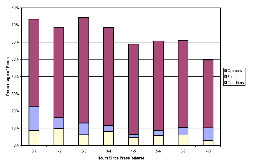
7.10.2 Breakdown of News Flow
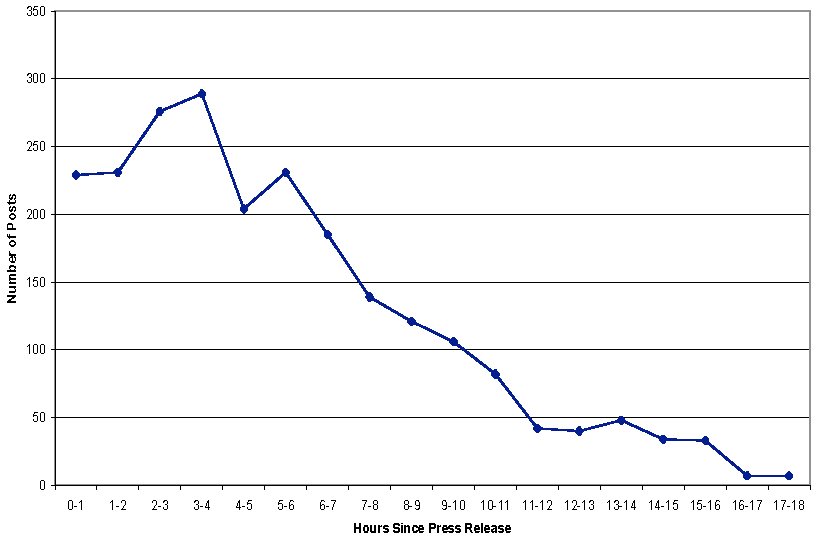
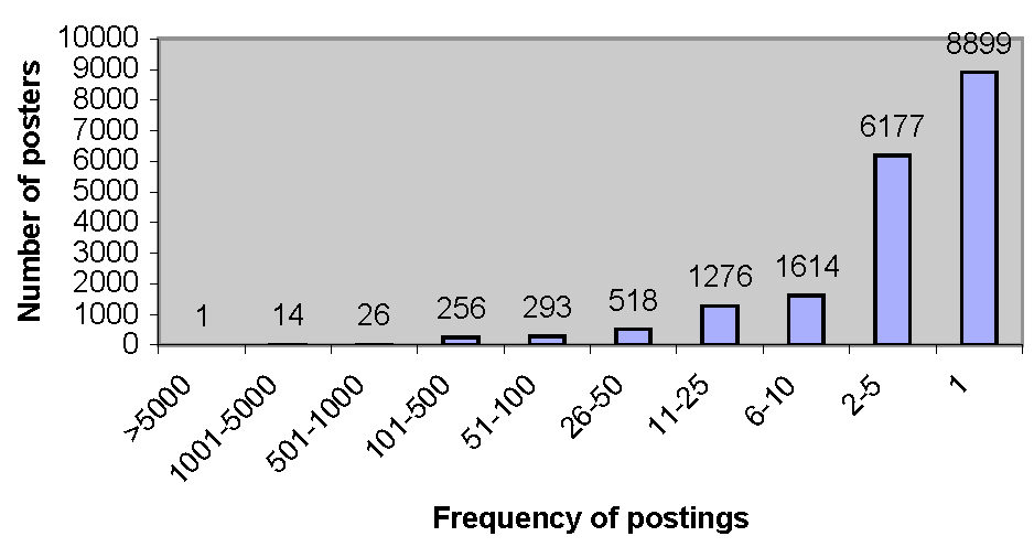
7.10.3 Frequency of Postings
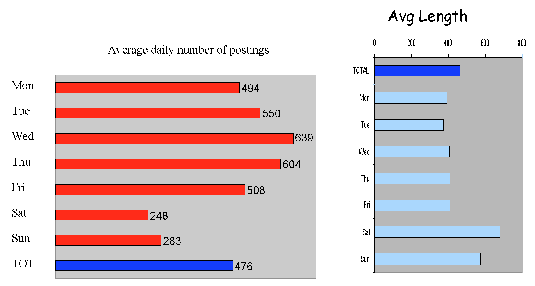
7.10.4 Weekly Posting
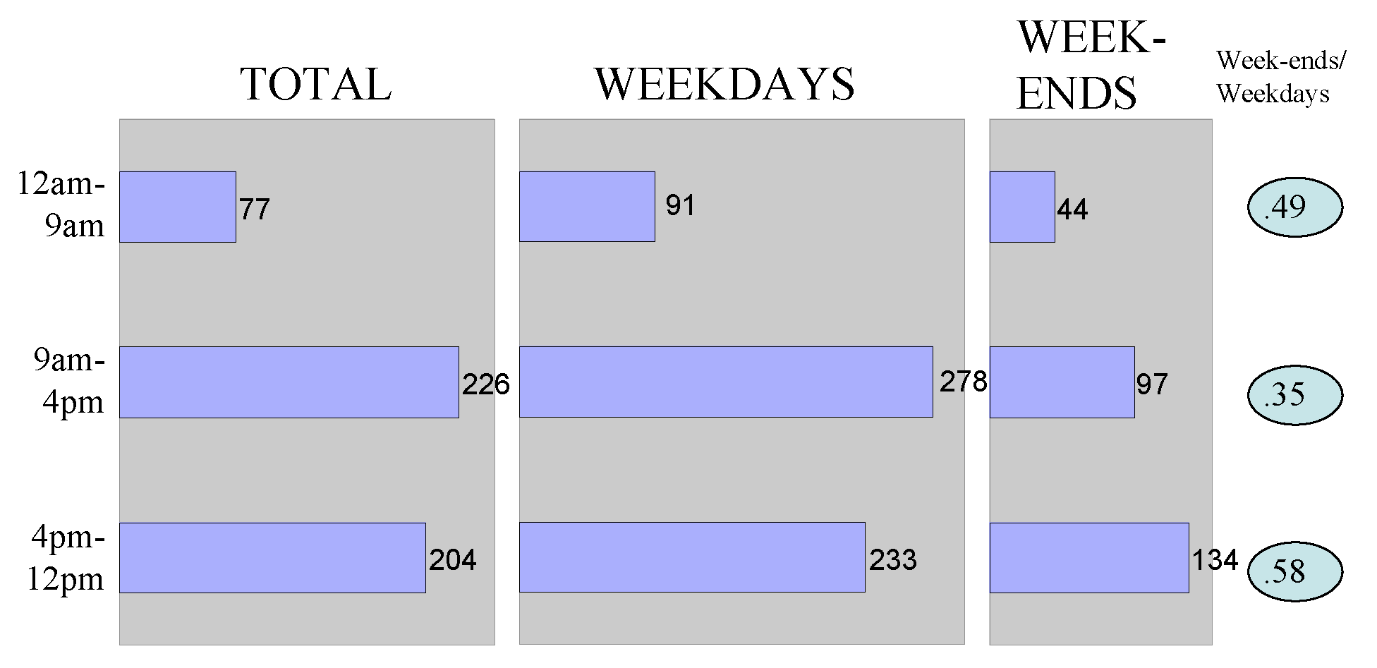
7.10.5 Intraday Posting
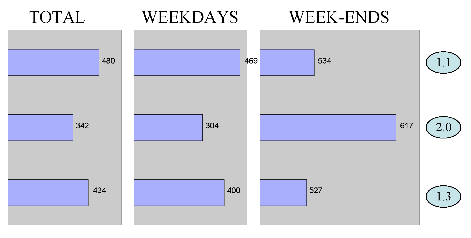
7.10.6 Number of Characters per Posting
7.11 Text Handling
First, let’s read in a simple web page (my landing page)
text = readLines("http://srdas.github.io/")
print(text[1:4])
## [1] "<html>"
## [2] ""
## [3] "<head>"
## [4] "<title>SCU Web Page of Sanjiv Ranjan Das</title>"print(length(text))## [1] 367.11.1 String Detection
String handling is a basic need, so we use the stringr package.
#EXTRACTING SUBSTRINGS (take some time to look at
#the "stringr" package also)
library(stringr)
substr(text[4],24,29)
## [1] "Sanjiv"#IF YOU WANT TO LOCATE A STRING
res = regexpr("Sanjiv",text[4])
print(res)## [1] 24
## attr(,"match.length")
## [1] 6
## attr(,"useBytes")
## [1] TRUEprint(substr(text[4],res[1],res[1]+nchar("Sanjiv")-1))## [1] "Sanjiv"#ANOTHER WAY
res = str_locate(text[4],"Sanjiv")
print(res)## start end
## [1,] 24 29print(substr(text[4],res[1],res[2]))## [1] "Sanjiv"7.11.2 Cleaning Text
Now we look at using regular expressions with the grep command to clean out text. I will read in my research page to process this. Here we are undertaking a “ruthless” cleanup.
#SIMPLE TEXT HANDLING
text = readLines("http://srdas.github.io/research.htm")
print(length(text))
## [1] 845#print(text)
text = text[setdiff(seq(1,length(text)),grep("<",text))]
text = text[setdiff(seq(1,length(text)),grep(">",text))]
text = text[setdiff(seq(1,length(text)),grep("]",text))]
text = text[setdiff(seq(1,length(text)),grep("}",text))]
text = text[setdiff(seq(1,length(text)),grep("_",text))]
text = text[setdiff(seq(1,length(text)),grep("\\/",text))]
print(length(text))## [1] 350#print(text)
text = str_replace_all(text,"[\"]","")
idx = which(nchar(text)==0)
research = text[setdiff(seq(1,length(text)),idx)]
print(research)## [1] "Data Science: Theories, Models, Algorithms, and Analytics (web book -- work in progress)"
## [2] "Derivatives: Principles and Practice (2010),"
## [3] "(Rangarajan Sundaram and Sanjiv Das), McGraw Hill."
## [4] "An Index-Based Measure of Liquidity,'' (with George Chacko and Rong Fan), (2016)."
## [5] "Matrix Metrics: Network-Based Systemic Risk Scoring, (2016)."
## [6] "of systemic risk. This paper won the First Prize in the MIT-CFP competition 2016 for "
## [7] "the best paper on SIFIs (systemically important financial institutions). "
## [8] "It also won the best paper award at "
## [9] "Credit Spreads with Dynamic Debt (with Seoyoung Kim), (2015), "
## [10] "Text and Context: Language Analytics for Finance, (2014),"
## [11] "Strategic Loan Modification: An Options-Based Response to Strategic Default,"
## [12] "Options and Structured Products in Behavioral Portfolios, (with Meir Statman), (2013), "
## [13] "and barrier range notes, in the presence of fat-tailed outcomes using copulas."
## [14] "Polishing Diamonds in the Rough: The Sources of Syndicated Venture Performance, (2011), (with Hoje Jo and Yongtae Kim), "
## [15] "Optimization with Mental Accounts, (2010), (with Harry Markowitz, Jonathan"
## [16] "Accounting-based versus market-based cross-sectional models of CDS spreads, "
## [17] "(with Paul Hanouna and Atulya Sarin), (2009), "
## [18] "Hedging Credit: Equity Liquidity Matters, (with Paul Hanouna), (2009),"
## [19] "An Integrated Model for Hybrid Securities,"
## [20] "Yahoo for Amazon! Sentiment Extraction from Small Talk on the Web,"
## [21] "Common Failings: How Corporate Defaults are Correlated "
## [22] "(with Darrell Duffie, Nikunj Kapadia and Leandro Saita)."
## [23] "A Clinical Study of Investor Discussion and Sentiment, "
## [24] "(with Asis Martinez-Jerez and Peter Tufano), 2005, "
## [25] "International Portfolio Choice with Systemic Risk,"
## [26] "The loss resulting from diminished diversification is small, while"
## [27] "Speech: Signaling, Risk-sharing and the Impact of Fee Structures on"
## [28] "investor welfare. Contrary to regulatory intuition, incentive structures"
## [29] "A Discrete-Time Approach to No-arbitrage Pricing of Credit derivatives"
## [30] "with Rating Transitions, (with Viral Acharya and Rangarajan Sundaram),"
## [31] "Pricing Interest Rate Derivatives: A General Approach,''(with George Chacko),"
## [32] "A Discrete-Time Approach to Arbitrage-Free Pricing of Credit Derivatives,'' "
## [33] "The Psychology of Financial Decision Making: A Case"
## [34] "for Theory-Driven Experimental Enquiry,''"
## [35] "1999, (with Priya Raghubir),"
## [36] "Of Smiles and Smirks: A Term Structure Perspective,''"
## [37] "A Theory of Banking Structure, 1999, (with Ashish Nanda),"
## [38] "by function based upon two dimensions: the degree of information asymmetry "
## [39] "A Theory of Optimal Timing and Selectivity,'' "
## [40] "A Direct Discrete-Time Approach to"
## [41] "Poisson-Gaussian Bond Option Pricing in the Heath-Jarrow-Morton "
## [42] "The Central Tendency: A Second Factor in"
## [43] "Bond Yields, 1998, (with Silverio Foresi and Pierluigi Balduzzi), "
## [44] "Efficiency with Costly Information: A Reinterpretation of"
## [45] "Evidence from Managed Portfolios, (with Edwin Elton, Martin Gruber and Matt "
## [46] "Presented and Reprinted in the Proceedings of The "
## [47] "Seminar on the Analysis of Security Prices at the Center "
## [48] "for Research in Security Prices at the University of "
## [49] "Managing Rollover Risk with Capital Structure Covenants"
## [50] "in Structured Finance Vehicles (2016),"
## [51] "The Design and Risk Management of Structured Finance Vehicles (2016),"
## [52] "Post the recent subprime financial crisis, we inform the creation of safer SIVs "
## [53] "in structured finance, and propose avenues of mitigating risks faced by senior debt through "
## [54] "Coming up Short: Managing Underfunded Portfolios in an LDI-ES Framework (2014), "
## [55] "(with Seoyoung Kim and Meir Statman), "
## [56] "Going for Broke: Restructuring Distressed Debt Portfolios (2014),"
## [57] "Digital Portfolios. (2013), "
## [58] "Options on Portfolios with Higher-Order Moments, (2009),"
## [59] "options on a multivariate system of assets, calibrated to the return "
## [60] "Dealing with Dimension: Option Pricing on Factor Trees, (2009),"
## [61] "you to price options on multiple assets in a unified fraamework. Computational"
## [62] "Modeling"
## [63] "Correlated Default with a Forest of Binomial Trees, (2007), (with"
## [64] "Basel II: Correlation Related Issues (2007), "
## [65] "Correlated Default Risk, (2006),"
## [66] "(with Laurence Freed, Gary Geng, and Nikunj Kapadia),"
## [67] "increase as markets worsen. Regime switching models are needed to explain dynamic"
## [68] "A Simple Model for Pricing Equity Options with Markov"
## [69] "Switching State Variables (2006),"
## [70] "(with Donald Aingworth and Rajeev Motwani),"
## [71] "The Firm's Management of Social Interactions, (2005)"
## [72] "(with D. Godes, D. Mayzlin, Y. Chen, S. Das, C. Dellarocas, "
## [73] "B. Pfeieffer, B. Libai, S. Sen, M. Shi, and P. Verlegh). "
## [74] "Financial Communities (with Jacob Sisk), 2005, "
## [75] "Summer, 112-123."
## [76] "Monte Carlo Markov Chain Methods for Derivative Pricing"
## [77] "and Risk Assessment,(with Alistair Sinclair), 2005, "
## [78] "where incomplete information about the value of an asset may be exploited to "
## [79] "undertake fast and accurate pricing. Proof that a fully polynomial randomized "
## [80] "Correlated Default Processes: A Criterion-Based Copula Approach,"
## [81] "Special Issue on Default Risk. "
## [82] "Private Equity Returns: An Empirical Examination of the Exit of"
## [83] "Venture-Backed Companies, (with Murali Jagannathan and Atulya Sarin),"
## [84] "firm being financed, the valuation at the time of financing, and the prevailing market"
## [85] "sentiment. Helps understand the risk premium required for the"
## [86] "Issue on Computational Methods in Economics and Finance), "
## [87] "December, 55-69."
## [88] "Bayesian Migration in Credit Ratings Based on Probabilities of"
## [89] "The Impact of Correlated Default Risk on Credit Portfolios,"
## [90] "(with Gifford Fong, and Gary Geng),"
## [91] "How Diversified are Internationally Diversified Portfolios:"
## [92] "Time-Variation in the Covariances between International Returns,"
## [93] "Discrete-Time Bond and Option Pricing for Jump-Diffusion"
## [94] "Macroeconomic Implications of Search Theory for the Labor Market,"
## [95] "Auction Theory: A Summary with Applications and Evidence"
## [96] "from the Treasury Markets, 1996, (with Rangarajan Sundaram),"
## [97] "A Simple Approach to Three Factor Affine Models of the"
## [98] "Term Structure, (with Pierluigi Balduzzi, Silverio Foresi and Rangarajan"
## [99] "Analytical Approximations of the Term Structure"
## [100] "for Jump-diffusion Processes: A Numerical Analysis, 1996, "
## [101] "Markov Chain Term Structure Models: Extensions and Applications,"
## [102] "Exact Solutions for Bond and Options Prices"
## [103] "with Systematic Jump Risk, 1996, (with Silverio Foresi),"
## [104] "Pricing Credit Sensitive Debt when Interest Rates, Credit Ratings"
## [105] "and Credit Spreads are Stochastic, 1996, "
## [106] "v5(2), 161-198."
## [107] "Did CDS Trading Improve the Market for Corporate Bonds, (2016), "
## [108] "(with Madhu Kalimipalli and Subhankar Nayak), "
## [109] "Big Data's Big Muscle, (2016), "
## [110] "Portfolios for Investors Who Want to Reach Their Goals While Staying on the Mean-Variance Efficient Frontier, (2011), "
## [111] "(with Harry Markowitz, Jonathan Scheid, and Meir Statman), "
## [112] "News Analytics: Framework, Techniques and Metrics, The Handbook of News Analytics in Finance, May 2011, John Wiley & Sons, U.K. "
## [113] "Random Lattices for Option Pricing Problems in Finance, (2011),"
## [114] "Implementing Option Pricing Models using Python and Cython, (2010),"
## [115] "The Finance Web: Internet Information and Markets, (2010), "
## [116] "Financial Applications with Parallel R, (2009), "
## [117] "Recovery Swaps, (2009), (with Paul Hanouna), "
## [118] "Recovery Rates, (2009),(with Paul Hanouna), "
## [119] "``A Simple Model for Pricing Securities with a Debt-Equity Linkage,'' 2008, in "
## [120] "Credit Default Swap Spreads, 2006, (with Paul Hanouna), "
## [121] "Multiple-Core Processors for Finance Applications, 2006, "
## [122] "Power Laws, 2005, (with Jacob Sisk), "
## [123] "Genetic Algorithms, 2005,"
## [124] "Recovery Risk, 2005,"
## [125] "Venture Capital Syndication, (with Hoje Jo and Yongtae Kim), 2004"
## [126] "Technical Analysis, (with David Tien), 2004"
## [127] "Liquidity and the Bond Markets, (with Jan Ericsson and "
## [128] "Madhu Kalimipalli), 2003,"
## [129] "Modern Pricing of Interest Rate Derivatives - Book Review, "
## [130] "Contagion, 2003,"
## [131] "Hedge Funds, 2003,"
## [132] "Reprinted in "
## [133] "Working Papers on Hedge Funds, in The World of Hedge Funds: "
## [134] "Characteristics and "
## [135] "Analysis, 2005, World Scientific."
## [136] "The Internet and Investors, 2003,"
## [137] " Useful things to know about Correlated Default Risk,"
## [138] "(with Gifford Fong, Laurence Freed, Gary Geng, and Nikunj Kapadia),"
## [139] "The Regulation of Fee Structures in Mutual Funds: A Theoretical Analysis,'' "
## [140] "(with Rangarajan Sundaram), 1998, NBER WP No 6639, in the"
## [141] "Courant Institute of Mathematical Sciences, special volume on"
## [142] "A Discrete-Time Approach to Arbitrage-Free Pricing of Credit Derivatives,'' "
## [143] "(with Rangarajan Sundaram), reprinted in "
## [144] "the Courant Institute of Mathematical Sciences, special volume on"
## [145] "Stochastic Mean Models of the Term Structure,''"
## [146] "(with Pierluigi Balduzzi, Silverio Foresi and Rangarajan Sundaram), "
## [147] "John Wiley & Sons, Inc., 128-161."
## [148] "Interest Rate Modeling with Jump-Diffusion Processes,'' "
## [149] "John Wiley & Sons, Inc., 162-189."
## [150] "Comments on 'Pricing Excess-of-Loss Reinsurance Contracts against"
## [151] "Catastrophic Loss,' by J. David Cummins, C. Lewis, and Richard Phillips,"
## [152] "Froot (Ed.), University of Chicago Press, 1999, 141-145."
## [153] " Pricing Credit Derivatives,'' "
## [154] "J. Frost and J.G. Whittaker, 101-138."
## [155] "On the Recursive Implementation of Term Structure Models,'' "
## [156] "Zero-Revelation RegTech: Detecting Risk through"
## [157] "Linguistic Analysis of Corporate Emails and News "
## [158] "(with Seoyoung Kim and Bhushan Kothari)."
## [159] "Summary for the Columbia Law School blog: "
## [160] " "
## [161] "Dynamic Risk Networks: A Note "
## [162] "(with Seoyoung Kim and Dan Ostrov)."
## [163] "Research Challenges in Financial Data Modeling and Analysis "
## [164] "(with Lewis Alexander, Zachary Ives, H.V. Jagadish, and Claire Monteleoni)."
## [165] "Local Volatility and the Recovery Rate of Credit Default Swaps "
## [166] "(with Jeroen Jansen and Frank Fabozzi)."
## [167] "Efficient Rebalancing of Taxable Portfolios (with Dan Ostrov, Dennis Ding, Vincent Newell), "
## [168] "The Fast and the Curious: VC Drift "
## [169] "(with Amit Bubna and Paul Hanouna), "
## [170] "Venture Capital Communities (with Amit Bubna and Nagpurnanand Prabhala), "
## [171] " "Take a look at the text now to see how cleaned up it is. But there is a better way, i.e., use the text-mining package tm.
7.12 Package tm
The R programming language supports a text-mining package, succinctly named {tm}. Using functions such as {readDOC()}, {readPDF()}, etc., for reading DOC and PDF files, the package makes accessing various file formats easy.
Text mining involves applying functions to many text documents. A library of text documents (irrespective of format) is called a corpus. The essential and highly useful feature of text mining packages is the ability to operate on the entire set of documents at one go.
library(tm)## Loading required package: NLPtext = c("INTL is expected to announce good earnings report", "AAPL first quarter disappoints","GOOG announces new wallet", "YHOO ascends from old ways")
text_corpus = Corpus(VectorSource(text))
print(text_corpus)## <<VCorpus>>
## Metadata: corpus specific: 0, document level (indexed): 0
## Content: documents: 4writeCorpus(text_corpus)The writeCorpus() function in tm creates separate text files on the hard drive, and by default are names 1.txt, 2.txt, etc. The simple program code above shows how text scraped off a web page and collapsed into a single character string for each document, may then be converted into a corpus of documents using the Corpus() function.
It is easy to inspect the corpus as follows:
inspect(text_corpus)## <<VCorpus>>
## Metadata: corpus specific: 0, document level (indexed): 0
## Content: documents: 4
##
## [[1]]
## <<PlainTextDocument>>
## Metadata: 7
## Content: chars: 49
##
## [[2]]
## <<PlainTextDocument>>
## Metadata: 7
## Content: chars: 30
##
## [[3]]
## <<PlainTextDocument>>
## Metadata: 7
## Content: chars: 25
##
## [[4]]
## <<PlainTextDocument>>
## Metadata: 7
## Content: chars: 267.12.1 A second example
Here we use lapply to inspect the contents of the corpus.
#USING THE tm PACKAGE
library(tm)
text = c("Doc1;","This is doc2 --", "And, then Doc3.")
ctext = Corpus(VectorSource(text))
ctext
## <<VCorpus>>
## Metadata: corpus specific: 0, document level (indexed): 0
## Content: documents: 3#writeCorpus(ctext)
#THE CORPUS IS A LIST OBJECT in R of type VCorpus or Corpus
inspect(ctext)## <<VCorpus>>
## Metadata: corpus specific: 0, document level (indexed): 0
## Content: documents: 3
##
## [[1]]
## <<PlainTextDocument>>
## Metadata: 7
## Content: chars: 5
##
## [[2]]
## <<PlainTextDocument>>
## Metadata: 7
## Content: chars: 15
##
## [[3]]
## <<PlainTextDocument>>
## Metadata: 7
## Content: chars: 15print(as.character(ctext[[1]]))## [1] "Doc1;"print(lapply(ctext[1:2],as.character))## $`1`
## [1] "Doc1;"
##
## $`2`
## [1] "This is doc2 --"ctext = tm_map(ctext,tolower) #Lower case all text in all docs
inspect(ctext)## <<VCorpus>>
## Metadata: corpus specific: 0, document level (indexed): 0
## Content: documents: 3
##
## [[1]]
## [1] doc1;
##
## [[2]]
## [1] this is doc2 --
##
## [[3]]
## [1] and, then doc3.ctext2 = tm_map(ctext,toupper)
inspect(ctext2)## <<VCorpus>>
## Metadata: corpus specific: 0, document level (indexed): 0
## Content: documents: 3
##
## [[1]]
## [1] DOC1;
##
## [[2]]
## [1] THIS IS DOC2 --
##
## [[3]]
## [1] AND, THEN DOC3.7.12.2 Function tm_map
- The tm_map function is very useful for cleaning up the documents. We may want to remove some words.
- We may also remove stopwords, punctuation, numbers, etc.
#FIRST CURATE TO UPPER CASE
dropWords = c("IS","AND","THEN")
ctext2 = tm_map(ctext2,removeWords,dropWords)
inspect(ctext2)
## <<VCorpus>>
## Metadata: corpus specific: 0, document level (indexed): 0
## Content: documents: 3
##
## [[1]]
## [1] DOC1;
##
## [[2]]
## [1] THIS DOC2 --
##
## [[3]]
## [1] , DOC3.ctext = Corpus(VectorSource(text))
temp = ctext
print(lapply(temp,as.character))## $`1`
## [1] "Doc1;"
##
## $`2`
## [1] "This is doc2 --"
##
## $`3`
## [1] "And, then Doc3."temp = tm_map(temp,removeWords,stopwords("english"))
print(lapply(temp,as.character))## $`1`
## [1] "Doc1;"
##
## $`2`
## [1] "This doc2 --"
##
## $`3`
## [1] "And, Doc3."temp = tm_map(temp,removePunctuation)
print(lapply(temp,as.character))## $`1`
## [1] "Doc1"
##
## $`2`
## [1] "This doc2 "
##
## $`3`
## [1] "And Doc3"temp = tm_map(temp,removeNumbers)
print(lapply(temp,as.character))## $`1`
## [1] "Doc"
##
## $`2`
## [1] "This doc "
##
## $`3`
## [1] "And Doc"7.12.3 Bag of Words
We can create a bag of words by collapsing all the text into one bundle.
#CONVERT CORPUS INTO ARRAY OF STRINGS AND FLATTEN
txt = NULL
for (j in 1:length(temp)) {
  txt = c(txt,temp[[j]]$content)
}
txt = paste(txt,collapse=" ")
txt = tolower(txt)
print(txt)
## [1] "doc this doc and doc"7.12.4 Example (on my bio page)
Now we will do a full pass through of this on my bio.
text = readLines("http://srdas.github.io/bio-candid.html")
ctext = Corpus(VectorSource(text))
ctext
## <<VCorpus>>
## Metadata: corpus specific: 0, document level (indexed): 0
## Content: documents: 80#Print a few lines
print(lapply(ctext, as.character)[10:15])## $`10`
## [1] "B.Com in Accounting and Economics (University of Bombay, Sydenham"
##
## $`11`
## [1] "College), and is also a qualified Cost and Works Accountant"
##
## $`12`
## [1] "(AICWA). He is a senior editor of The Journal of Investment"
##
## $`13`
## [1] "Management, co-editor of The Journal of Derivatives and The Journal of"
##
## $`14`
## [1] "Financial Services Research, and Associate Editor of other academic"
##
## $`15`
## [1] "journals. Prior to being an academic, he worked in the derivatives"ctext = tm_map(ctext,removePunctuation)
print(lapply(ctext, as.character)[10:15])## $`10`
## [1] "BCom in Accounting and Economics University of Bombay Sydenham"
##
## $`11`
## [1] "College and is also a qualified Cost and Works Accountant"
##
## $`12`
## [1] "AICWA He is a senior editor of The Journal of Investment"
##
## $`13`
## [1] "Management coeditor of The Journal of Derivatives and The Journal of"
##
## $`14`
## [1] "Financial Services Research and Associate Editor of other academic"
##
## $`15`
## [1] "journals Prior to being an academic he worked in the derivatives"txt = NULL
for (j in 1:length(ctext)) {
txt = c(txt,ctext[[j]]$content)
}
txt = paste(txt,collapse=" ")
txt = tolower(txt)
print(txt)## [1] "html body backgroundhttpalgoscuedusanjivdasgraphicsback2gif sanjiv das is the william and janice terry professor of finance at santa clara universitys leavey school of business he previously held faculty appointments as associate professor at harvard business school and uc berkeley he holds postgraduate degrees in finance mphil and phd from new york university computer science ms from uc berkeley an mba from the indian institute of management ahmedabad bcom in accounting and economics university of bombay sydenham college and is also a qualified cost and works accountant aicwa he is a senior editor of the journal of investment management coeditor of the journal of derivatives and the journal of financial services research and associate editor of other academic journals prior to being an academic he worked in the derivatives business in the asiapacific region as a vicepresident at citibank his current research interests include machine learning social networks derivatives pricing models portfolio theory the modeling of default risk and venture capital he has published over ninety articles in academic journals and has won numerous awards for research and teaching his recent book derivatives principles and practice was published in may 2010 second edition 2016 he currently also serves as a senior fellow at the fdic center for financial research p bsanjiv das a short academic life historyb p after loafing and working in many parts of asia but never really growing up sanjiv moved to new york to change the world hopefully through research he graduated in 1994 with a phd from nyu and since then spent five years in boston and now lives in san jose california sanjiv loves animals places in the world where the mountains meet the sea riding sport motorbikes reading gadgets science fiction movies and writing cool software code when there is time available from the excitement of daily life sanjiv writes academic papers which helps him relax always the contrarian sanjiv thinks that new york city is the most calming place in the world after california of course p sanjiv is now a professor of finance at santa clara university he came to scu from harvard business school and spent a year at uc berkeley in his past life in the unreal world sanjiv worked at citibank na in the asiapacific region he takes great pleasure in merging his many previous lives into his current existence which is incredibly confused and diverse p sanjivs research style is instilled with a distinct new york state of mind it is chaotic diverse with minimal method to the madness he has published articles on derivatives termstructure models mutual funds the internet portfolio choice banking models credit risk and has unpublished articles in many other areas some years ago he took time off to get another degree in computer science at berkeley confirming that an unchecked hobby can quickly become an obsession there he learnt about the fascinating field of randomized algorithms skills he now applies earnestly to his editorial work and other pursuits many of which stem from being in the epicenter of silicon valley p coastal living did a lot to mold sanjiv who needs to live near the ocean the many walks in greenwich village convinced him that there is no such thing as a representative investor yet added many unique features to his personal utility function he learnt that it is important to open the academic door to the ivory tower and let the world in academia is a real challenge given that he has to reconcile many more opinions than ideas he has been known to have turned down many offers from mad magazine to publish his academic work as he often explains you never really finish your education you can check out any time you like but you can never leave which is why he is doomed to a lifetime in hotel california and he believes that if this is as bad as it gets life is really pretty good "7.13 Term Document Matrix (TDM)
An extremeley important object in text analysis is the Term-Document Matrix. This allows us to store an entire library of text inside a single matrix. This may then be used for analysis as well as searching documents. It forms the basis of search engines, topic analysis, and classification (spam filtering).
It is a table that provides the frequency count of every word (term) in each document. The number of rows in the TDM is equal to the number of unique terms, and the number of columns is equal to the number of documents.
#TERM-DOCUMENT MATRIX
tdm = TermDocumentMatrix(ctext,control=list(minWordLength=1))
print(tdm)
## <<TermDocumentMatrix (terms: 321, documents: 80)>>
## Non-/sparse entries: 502/25178
## Sparsity : 98%
## Maximal term length: 49
## Weighting : term frequency (tf)inspect(tdm[10:20,11:18])## <<TermDocumentMatrix (terms: 11, documents: 8)>>
## Non-/sparse entries: 5/83
## Sparsity : 94%
## Maximal term length: 10
## Weighting : term frequency (tf)
##
## Docs
## Terms 11 12 13 14 15 16 17 18
## after 0 0 0 0 0 0 0 0
## ago 0 0 0 0 0 0 0 0
## ahmedabad 0 0 0 0 0 0 0 0
## aicwa 0 1 0 0 0 0 0 0
## algorithms 0 0 0 0 0 0 0 0
## also 1 0 0 0 0 0 0 0
## always 0 0 0 0 0 0 0 0
## and 2 0 1 1 0 0 0 0
## animals 0 0 0 0 0 0 0 0
## another 0 0 0 0 0 0 0 0
## any 0 0 0 0 0 0 0 0out = findFreqTerms(tdm,lowfreq=5)
print(out)## [1] "academic" "and" "derivatives" "from" "has"
## [6] "his" "many" "research" "sanjiv" "that"
## [11] "the" "world"7.14 Term Frequency - Inverse Document Frequency (TF-IDF)
This is a weighting scheme provided to sharpen the importance of rare words in a document, relative to the frequency of these words in the corpus. It is based on simple calculations and even though it does not have strong theoretical foundations, it is still very useful in practice. The TF-IDF is the importance of a word \(w\) in a document \(d\) in a corpus \(C\). Therefore it is a function of all these three, i.e., we write it as TF-IDF\((w,d,C)\), and is the product of term frequency (TF) and inverse document frequency (IDF).
The frequency of a word in a document is defined as
\[ f(w,d) = \frac{\#w \in d}{|d|} \]
where \(|d|\) is the number of words in the document. We usually normalize word frequency so that
\[ TF(w,d) = \ln[f(w,d)] \] This is log normalization. Another form of normalization is known as double normalization and is as follows:
\[ TF(w,d) = \frac{1}{2} + \frac{1}{2} \frac{f(w,d)}{\max_{w \in d} f(w,d)} \]
Note that normalization is not necessary, but it tends to help shrink the difference between counts of words.
Inverse document frequency is as follows:
\[ IDF(w,C) = \ln\left[ \frac{|C|}{|d_{w \in d}|} \right] \] That is, we compute the ratio of the number of documents in the corpus \(C\) divided by the number of documents with word \(w\) in the corpus.
Finally, we have the weighting score for a given word \(w\) in document \(d\) in corpus \(C\):
\[ \mbox{TF-IDF}(w,d,C) = TF(w,d) \times IDF(w,C) \]
7.14.1 Example of TD-IDF
We illustrate this with an application to the previously computed term-document matrix.
tdm_mat = as.matrix(tdm)  #Convert tdm into a matrix
print(dim(tdm_mat))
## [1] 321 80nw = dim(tdm_mat)[1]
nd = dim(tdm_mat)[2]
doc = 13 #Choose document
word = "derivatives" #Choose word
#COMPUTE TF
f = NULL
for (w in row.names(tdm_mat)) {
f = c(f,tdm_mat[w,doc]/sum(tdm_mat[,doc]))
}
fw = tdm_mat[word,doc]/sum(tdm_mat[,doc])
TF = 0.5 + 0.5*fw/max(f)
print(TF)## [1] 0.75#COMPUTE IDF
nw = length(which(tdm_mat[word,]>0))
print(nw)## [1] 5IDF = nd/nw
print(IDF)## [1] 16#COMPUTE TF-IDF
TF_IDF = TF*IDF
print(TF_IDF) #With normalization## [1] 12print(fw*IDF) #Without normalization## [1] 2We can write this code into a function and work out the TF-IDF for all words. Then these word weights may be used in further text analysis.
7.14.2 TF-IDF in the tm package
We may also directly use the weightTfIdf function in the tm package. This undertakes the following computation:
Term frequency \({\it tf}_{i,j}\) counts the number of occurrences \(n_{i,j}\) of a term \(t_i\) in a document \(d_j\). In the case of normalization, the term frequency \(\mathit{tf}_{i,j}\) is divided by \(\sum_k n_{k,j}\).
Inverse document frequency for a term \(t_i\) is defined as \(\mathit{idf}_i = \log_2 \frac{|D|}{|{d_{t_i \in d}}|}\) where \(|D|\) denotes the total number of documents \(|{d_{t_i \in d}}|\) is the number of documents where the term \(t_i\) appears.
Term frequency - inverse document frequency is now defined as \(\mathit{tf}_{i,j} \cdot \mathit{idf}_i\).
tdm = TermDocumentMatrix(ctext,control=list(minWordLength=1,weighting=weightTfIdf))## Warning in weighting(x): empty document(s): 3 25 26 28 40 41 42 49 50 51 63
## 64 65 78 79 80print(tdm)## <<TermDocumentMatrix (terms: 321, documents: 80)>>
## Non-/sparse entries: 502/25178
## Sparsity : 98%
## Maximal term length: 49
## Weighting : term frequency - inverse document frequency (normalized) (tf-idf)inspect(tdm[10:20,11:18])## <<TermDocumentMatrix (terms: 11, documents: 8)>>
## Non-/sparse entries: 5/83
## Sparsity : 94%
## Maximal term length: 10
## Weighting : term frequency - inverse document frequency (normalized) (tf-idf)
##
## Docs
## Terms 11 12 13 14 15 16 17 18
## after 0.0000000 0.000000 0.0000000 0.0000000 0 0 0 0
## ago 0.0000000 0.000000 0.0000000 0.0000000 0 0 0 0
## ahmedabad 0.0000000 0.000000 0.0000000 0.0000000 0 0 0 0
## aicwa 0.0000000 1.053655 0.0000000 0.0000000 0 0 0 0
## algorithms 0.0000000 0.000000 0.0000000 0.0000000 0 0 0 0
## also 0.6652410 0.000000 0.0000000 0.0000000 0 0 0 0
## always 0.0000000 0.000000 0.0000000 0.0000000 0 0 0 0
## and 0.5185001 0.000000 0.2592501 0.2592501 0 0 0 0
## animals 0.0000000 0.000000 0.0000000 0.0000000 0 0 0 0
## another 0.0000000 0.000000 0.0000000 0.0000000 0 0 0 0
## any 0.0000000 0.000000 0.0000000 0.0000000 0 0 0 0Example:
library(tm)
textarray = c("Free software comes with ABSOLUTELY NO certain WARRANTY","You are welcome to redistribute free software under certain conditions","Natural language support for software in an English locale","A collaborative project with many contributors")
textcorpus = Corpus(VectorSource(textarray))
m = TermDocumentMatrix(textcorpus)
print(as.matrix(m))
## Docs
## Terms 1 2 3 4
## absolutely 1 0 0 0
## are 0 1 0 0
## certain 1 1 0 0
## collaborative 0 0 0 1
## comes 1 0 0 0
## conditions 0 1 0 0
## contributors 0 0 0 1
## english 0 0 1 0
## for 0 0 1 0
## free 1 1 0 0
## language 0 0 1 0
## locale 0 0 1 0
## many 0 0 0 1
## natural 0 0 1 0
## project 0 0 0 1
## redistribute 0 1 0 0
## software 1 1 1 0
## support 0 0 1 0
## under 0 1 0 0
## warranty 1 0 0 0
## welcome 0 1 0 0
## with 1 0 0 1
## you 0 1 0 0print(as.matrix(weightTfIdf(m)))## Docs
## Terms 1 2 3 4
## absolutely 0.28571429 0.00000000 0.00000000 0.0
## are 0.00000000 0.22222222 0.00000000 0.0
## certain 0.14285714 0.11111111 0.00000000 0.0
## collaborative 0.00000000 0.00000000 0.00000000 0.4
## comes 0.28571429 0.00000000 0.00000000 0.0
## conditions 0.00000000 0.22222222 0.00000000 0.0
## contributors 0.00000000 0.00000000 0.00000000 0.4
## english 0.00000000 0.00000000 0.28571429 0.0
## for 0.00000000 0.00000000 0.28571429 0.0
## free 0.14285714 0.11111111 0.00000000 0.0
## language 0.00000000 0.00000000 0.28571429 0.0
## locale 0.00000000 0.00000000 0.28571429 0.0
## many 0.00000000 0.00000000 0.00000000 0.4
## natural 0.00000000 0.00000000 0.28571429 0.0
## project 0.00000000 0.00000000 0.00000000 0.4
## redistribute 0.00000000 0.22222222 0.00000000 0.0
## software 0.05929107 0.04611528 0.05929107 0.0
## support 0.00000000 0.00000000 0.28571429 0.0
## under 0.00000000 0.22222222 0.00000000 0.0
## warranty 0.28571429 0.00000000 0.00000000 0.0
## welcome 0.00000000 0.22222222 0.00000000 0.0
## with 0.14285714 0.00000000 0.00000000 0.2
## you 0.00000000 0.22222222 0.00000000 0.07.15 Cosine Similarity in the Text Domain
In this segment we will learn some popular functions on text that are used in practice. One of the first things we like to do is to find similar text or like sentences (think of web search as one application). Since documents are vectors in the TDM, we may want to find the closest vectors or compute the distance between vectors.
\[ cos(\theta) = \frac{A \cdot B}{||A|| \times ||B||} \]
where \(||A|| = \sqrt{A \cdot A}\), is the dot product of \(A\) with itself, also known as the norm of \(A\). This gives the cosine of the angle between the two vectors and is zero for orthogonal vectors and 1 for identical vectors.
#COSINE DISTANCE OR SIMILARITY
A = as.matrix(c(0,3,4,1,7,0,1))
B = as.matrix(c(0,4,3,0,6,1,1))
cos = t(A) %*% B / (sqrt(t(A)%*%A) * sqrt(t(B)%*%B))
print(cos)
## [,1]
## [1,] 0.9682728library(lsa)## Loading required package: SnowballC#THE COSINE FUNCTION IN LSA ONLY TAKES ARRAYS
A = c(0,3,4,1,7,0,1)
B = c(0,4,3,0,6,1,1)
print(cosine(A,B))## [,1]
## [1,] 0.96827287.16 Using the ANLP package for bigrams and trigrams
This package has a few additional functions that make the preceding ideas more streamlined to implement. First let’s read in the usual text.
library(ANLP)
download.file("http://srdas.github.io/bio-candid.html",destfile = "text")
text = readTextFile("text","UTF-8")
ctext = cleanTextData(text)  #Creates a text corpus
The last function removes non-english characters, numbers, white spaces, brackets, punctuation. It also handles cases like abbreviation, contraction. It converts entire text to lower case.
We now make TDMs for unigrams, bigrams, trigrams. Then, combine them all into one list for word prediction.
g1 = generateTDM(ctext,1)
g2 = generateTDM(ctext,2)
g3 = generateTDM(ctext,3)
gmodel = list(g1,g2,g3)
Next, use the back-off algorithm to predict the next sequence of words.
print(predict_Backoff("you never",gmodel))
print(predict_Backoff("life is",gmodel))
print(predict_Backoff("been known",gmodel))
print(predict_Backoff("needs to",gmodel))
print(predict_Backoff("worked at",gmodel))
print(predict_Backoff("being an",gmodel))
print(predict_Backoff("publish",gmodel))
7.17 Wordclouds
Wordlcouds are interesting ways in which to represent text. They give an instant visual summary. The wordcloud package in R may be used to create your own wordclouds.
#MAKE A WORDCLOUD
library(wordcloud)
## Loading required package: RColorBrewertdm2 = as.matrix(tdm)
wordcount = sort(rowSums(tdm2),decreasing=TRUE)
tdm_names = names(wordcount)
wordcloud(tdm_names,wordcount)## Warning in wordcloud(tdm_names, wordcount):
## backgroundhttpalgoscuedusanjivdasgraphicsback2gif could not be fit on page.
## It will not be plotted.
#REMOVE STOPWORDS, NUMBERS, STEMMING
ctext1 = tm_map(ctext,removeWords,stopwords("english"))
ctext1 = tm_map(ctext1, removeNumbers)
tdm = TermDocumentMatrix(ctext1,control=list(minWordLength=1))
tdm2 = as.matrix(tdm)
wordcount = sort(rowSums(tdm2),decreasing=TRUE)
tdm_names = names(wordcount)
wordcloud(tdm_names,wordcount)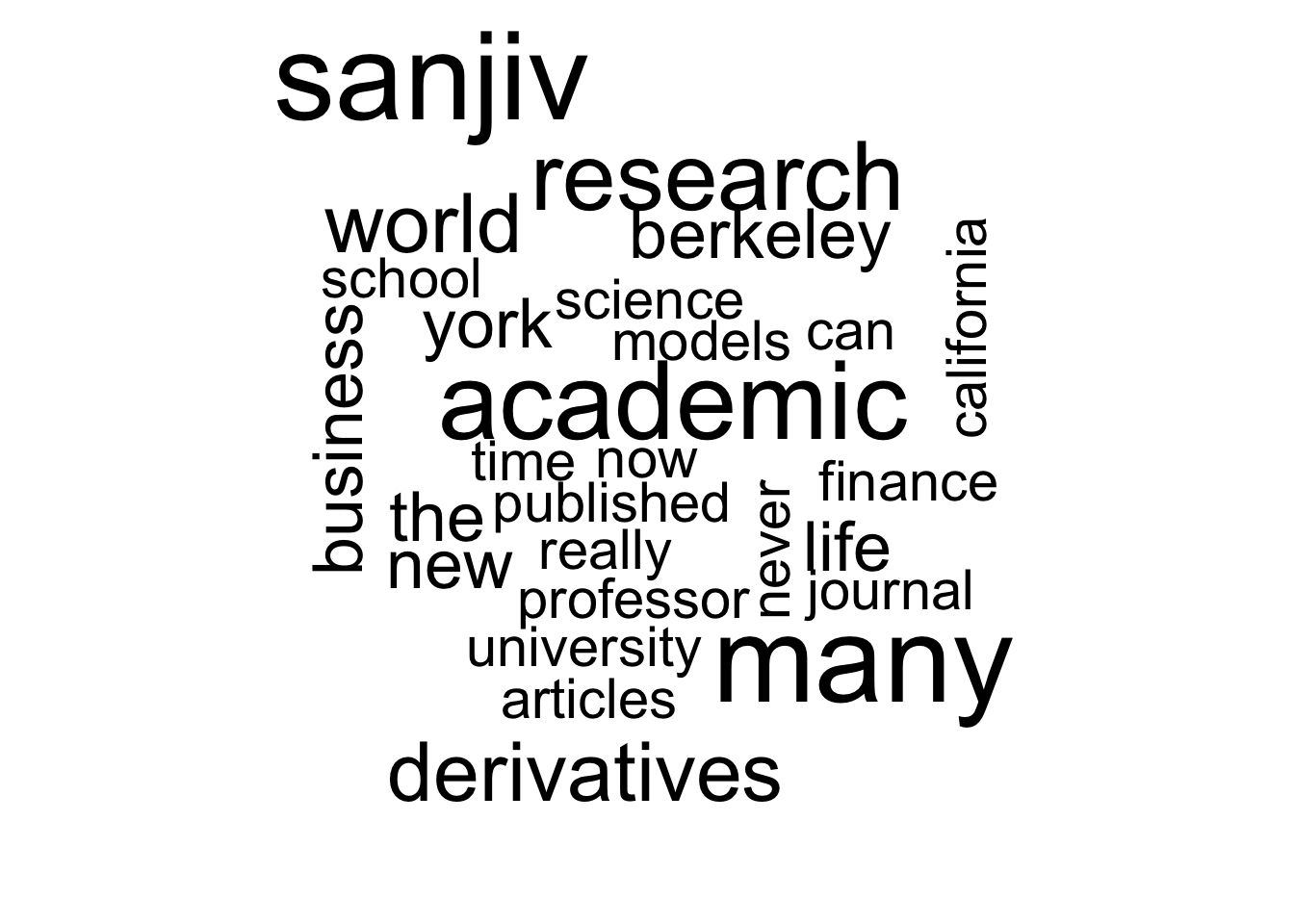
7.18 Manipulating Text
7.18.1 Stemming
Stemming is the procedure by which a word is reduced to its root or stem. This is done so as to treat words from the one stem as the same word, rather than as separate words. We do not want “eaten” and “eating” to be treated as different words for example.
#STEMMING
ctext2 = tm_map(ctext,removeWords,stopwords("english"))
ctext2 = tm_map(ctext2, stemDocument)
print(lapply(ctext2, as.character)[10:15])
## $`10`
## [1] "BCom Account Econom Univers Bombay Sydenham"
##
## $`11`
## [1] "Colleg also qualifi Cost Work Accountant"
##
## $`12`
## [1] "AICWA He senior editor The Journal Investment"
##
## $`13`
## [1] "Manag coeditor The Journal Deriv The Journal"
##
## $`14`
## [1] "Financi Servic Research Associat Editor academ"
##
## $`15`
## [1] "journal Prior academ work deriv"7.18.2 Regular Expressions
Regular expressions are syntax used to modify strings in an efficient manner. They are complicated but extremely effective. Here we will illustrate with a few examples, but you are encouraged to explore more on your own, as the variations are endless. What you need to do will depend on the application at hand, and with some experience you will become better at using regular expressions. The initial use will however be somewhat confusing.
We start with a simple example of a text array where we wish replace the string “data” with a blank, i.e., we eliminate this string from the text we have.
library(tm)
#Create a text array
text = c("Doc1 is datavision","Doc2 is datatable","Doc3 is data","Doc4 is nodata","Doc5 is simpler")
print(text)
## [1] "Doc1 is datavision" "Doc2 is datatable" "Doc3 is data"
## [4] "Doc4 is nodata" "Doc5 is simpler"#Remove all strings with the chosen text for all docs
print(gsub("data","",text))## [1] "Doc1 is vision" "Doc2 is table" "Doc3 is " "Doc4 is no"
## [5] "Doc5 is simpler"#Remove all words that contain "data" at the start even if they are longer than data
print(gsub("*data.*","",text))## [1] "Doc1 is " "Doc2 is " "Doc3 is " "Doc4 is no"
## [5] "Doc5 is simpler"#Remove all words that contain "data" at the end even if they are longer than data
print(gsub("*.data*","",text))## [1] "Doc1 isvision" "Doc2 istable" "Doc3 is" "Doc4 is n"
## [5] "Doc5 is simpler"#Remove all words that contain "data" at the end even if they are longer than data
print(gsub("*.data.*","",text))## [1] "Doc1 is" "Doc2 is" "Doc3 is" "Doc4 is n"
## [5] "Doc5 is simpler"7.18.3 Complex Regular Expressions using grep
We now explore some more complex regular expressions. One case that is common is handling the search for special types of strings like telephone numbers. Suppose we have a text array that may contain telephone numbers in different formats, we can use a single grep command to extract these numbers. Here is some code to illustrate this.
#Create an array with some strings which may also contain telephone numbers as strings.
x = c("234-5678","234 5678","2345678","1234567890","0123456789","abc 234-5678","234 5678 def","xx 2345678","abc1234567890def")

#Now use grep to find which elements of the array contain telephone numbers
idx = grep("[[:digit:]]{3}-[[:digit:]]{4}|[[:digit:]]{3} [[:digit:]]{4}|[1-9][0-9][0-9][0-9][0-9][0-9][0-9][0-9][0-9][0-9]",x)
print(idx)
## [1] 1 2 4 6 7 9print(x[idx])## [1] "234-5678" "234 5678" "1234567890"
## [4] "abc 234-5678" "234 5678 def" "abc1234567890def"#We can shorten this as follows
idx = grep("[[:digit:]]{3}-[[:digit:]]{4}|[[:digit:]]{3} [[:digit:]]{4}|[1-9][0-9]{9}",x)
print(idx)## [1] 1 2 4 6 7 9print(x[idx])## [1] "234-5678" "234 5678" "1234567890"
## [4] "abc 234-5678" "234 5678 def" "abc1234567890def"#What if we want to extract only the phone number and drop the rest of the text?
pattern = "[[:digit:]]{3}-[[:digit:]]{4}|[[:digit:]]{3} [[:digit:]]{4}|[1-9][0-9]{9}"
print(regmatches(x, gregexpr(pattern,x)))## [[1]]
## [1] "234-5678"
##
## [[2]]
## [1] "234 5678"
##
## [[3]]
## character(0)
##
## [[4]]
## [1] "1234567890"
##
## [[5]]
## character(0)
##
## [[6]]
## [1] "234-5678"
##
## [[7]]
## [1] "234 5678"
##
## [[8]]
## character(0)
##
## [[9]]
## [1] "1234567890"#Or use the stringr package, which is a lot better
library(stringr)
str_extract(x,pattern)## [1] "234-5678" "234 5678" NA "1234567890" NA
## [6] "234-5678" "234 5678" NA "1234567890"7.18.4 Using grep for emails
Now we use grep to extract emails by looking for the “@” sign in the text string. We would proceed as in the following example.
x = c("sanjiv das","srdas@scu.edu","SCU","data@science.edu")
print(grep("\\@",x))
## [1] 2 4print(x[grep("\\@",x)])## [1] "srdas@scu.edu" "data@science.edu"You get the idea. Using the functions gsub, grep, regmatches, and gregexpr, you can manage most fancy string handling that is needed.
7.19 Web Extraction using the rvest package
The rvest package, written bu Hadley Wickham, is a powerful tool for extracting text from web pages. The package provides wrappers around the ‘xml2’ and ‘httr’ packages to make it easy to download, and then manipulate, HTML and XML. The package is best illustrated with some simple examples.
7.19.1 Program to read a web page using the selector gadget
The selector gadget ius a useful tool to be used in conjunction with the rvest package. It allows you to find the html tag in a web page that you need to pass to the program to parse the html page element you are interested in. Download from: http://selectorgadget.com/
Here is some code to read in the slashdot web page and gather the stories currently on their headlines.
library(rvest)## Loading required package: xml2##
## Attaching package: 'rvest'## The following object is masked from 'package:XML':
##
## xmlurl = "https://slashdot.org/"
doc.html = read_html(url)
text = doc.html %>% html_nodes(".story") %>% html_text()
text = gsub("[\t\n]","",text)
#text = paste(text, collapse=" ")
print(text[1:20])## [1] " Samsung's Calls For Industry To Embrace Its Battery Check Process as a New Standard Have Been Ignored (cnet.com) "
## [2] " Blinking Cursor Devours CPU Cycles in Visual Studio Code Editor (theregister.co.uk) 39"
## [3] " Alcohol Is Good for Your Heart -- Most of the Time (time.com) 58"
## [4] " App That Lets People Make Personalized Emojis Is the Fastest Growing App In Past Two Years (axios.com) 22"
## [5] " Americans' Shift To The Suburbs Sped Up Last Year (fivethirtyeight.com) 113"
## [6] " Some Of Hacker Group's Claims Of Having Access To 250M iCloud Accounts Aren't False (zdnet.com) 33"
## [7] " Amazon Wins $1.5 Billion Tax Dispute Over IRS (reuters.com) 63"
## [8] " Hollywood Producer Blames Rotten Tomatoes For Convincing People Not To See His Movie (vanityfair.com) 283"
## [9] " Sea Ice Extent Sinks To Record Lows At Both Poles (sciencedaily.com) 130"
## [10] " Molecule Kills Elderly Cells, Reduces Signs of Aging In Mice (sciencemag.org) 94"
## [11] " Red-Light Camera Grace Period Goes From 0.1 To 0.3 Seconds, Chicago To Lose $17 Million (arstechnica.com) 201"
## [12] " US Ordered 'Mandatory Social Media Check' For Visa Applicants Who Visited ISIS Territory (theverge.com) 177"
## [13] " Google Reducing Trust In Symantec Certificates Following Numerous Slip-Ups (bleepingcomputer.com) 63"
## [14] " Twitter Considers Premium Version After 11 Years As a Free Service (reuters.com) 81"
## [15] " Apple Explores Using An iPhone, iPad To Power a Laptop (appleinsider.com) 63"
## [16] NA
## [17] NA
## [18] NA
## [19] NA
## [20] NA7.19.2 Program to read a web table using the selector gadget
Sometimes we need to read a table embedded in a web page and this is also a simple exercise, which is undertaken also with rvest.
library(rvest)
url = "http://finance.yahoo.com/q?uhb=uhb2&fr=uh3_finance_vert_gs&type=2button&s=IBM"

doc.html = read_html(url)
table = doc.html %>% html_nodes("table") %>% html_table()

print(table)
## [[1]]
## X1 X2
## 1 NA Search
##
## [[2]]
## X1 X2
## 1 Previous Close 174.82
## 2 Open 175.12
## 3 Bid 174.80 x 300
## 4 Ask 174.99 x 300
## 5 Day's Range 173.94 - 175.50
## 6 52 Week Range 142.50 - 182.79
## 7 Volume 1,491,738
## 8 Avg. Volume 3,608,856
##
## [[3]]
## X1 X2
## 1 Market Cap 164.3B
## 2 Beta 0.87
## 3 PE Ratio (TTM) 14.07
## 4 EPS (TTM) N/A
## 5 Earnings Date N/A
## 6 Dividend & Yield 5.60 (3.20%)
## 7 Ex-Dividend Date N/A
## 8 1y Target Est N/ANote that this code extracted all the web tables in the Yahoo! Finance page and returned each one as a list item.
7.19.3 Program to read a web table into a data frame
Here we take note of some Russian language sites where we want to extract forex quotes and store them in a data frame.
library(rvest)

url1 <- "http://finance.i.ua/market/kiev/?type=1"  #Buy USD
url2 <- "http://finance.i.ua/market/kiev/?type=2"  #Sell USD

doc1.html = read_html(url1)
table1 = doc1.html %>% html_nodes("table") %>% html_table()
result1 = table1[[1]]
print(head(result1))
## X1 X2 X3 X4
## 1 Время Курс Сумма Телефон
## 2 13:03 0.462 250000 \u20bd +38 063 \nПоказать
## 3 13:07 27.0701 72000 $ +38 063 \nПоказать
## 4 19:05 27.11 2000 $ +38 068 \nПоказать
## 5 18:48 27.08 200000 $ +38 063 \nПоказать
## 6 18:44 27.08 100000 $ +38 096 \nПоказать
## X5
## 1 Район
## 2 м Дружбы народов
## 3 Обмен Валют Ленинградская пл
## 4 Центр. Могу подъехать.
## 5 Леси Украинки. Дружба Народов. Лыбидская
## 6 Ленинградская Пл. Левобережка. Печерск
## X6
## 1 Комментарий
## 2 детектор, обмен валют
## 3 От 10т дол. Крупная гривна. От 30т нду. Звоните
## 4 Можно частями
## 5 П е ч е р с к , Подол. Лыбидская , от 10т. Обмен на Е В Р О 1. 0 82
## 6 П е ч е р с к , Подол. Лыбидская , от 10т. Обмен на Е В Р О 1. 082doc2.html = read_html(url2)
table2 = doc2.html %>% html_nodes("table") %>% html_table()
result2 = table2[[1]]
print(head(result2))## X1 X2 X3 X4
## 1 Время Курс Сумма Телефон
## 2 17:10 29.2299 62700 € +38 093 \nПоказать
## 3 19:04 27.14 5000 $ +38 098 \nПоказать
## 4 13:08 27.1099 72000 $ +38 063 \nПоказать
## 5 15:03 27.14 5200 $ +38 095 \nПоказать
## 6 17:05 27.2 40000 $ +38 093 \nПоказать
## X5
## 1 Район
## 2 Обменный пункт Ленинградская пл и
## 3 Центр. Подъеду
## 4 Обмен Валют Ленинградская пл
## 5 Печерск
## 6 Подол
## X6
## 1 Комментарий
## 2 Или за дол 1. 08 От 10т евро. 50 100 и 500 купюры. Звоните. Бронируйте. Еду от 10т. Артем
## 3 Можно Частями от 500 дол
## 4 От 10т дол. Крупная гривна. От 30т нду. Звоните
## 5 м Дружбы народов, от 500, детектор, обмен валют
## 6 Обмен валют, с 9-00 до 19-007.20 Using the rselenium package
#Clicking Show More button Google Scholar page

library(RCurl)
library(RSelenium)
library(rvest)
library(stringr)
library(igraph)
checkForServer()
startServer()
remDr <- remoteDriver(remoteServerAddr = "localhost"
                      , port = 4444
                      , browserName = "firefox"
)
remDr$open()
remDr$getStatus()
7.20.1 Application to Google Scholar data
remDr$navigate("http://scholar.google.com")
webElem <- remDr$findElement(using = 'css selector', "input#gs_hp_tsi")
webElem$sendKeysToElement(list("Sanjiv Das", "\uE007"))
link <- webElem$getCurrentUrl()
page <- read_html(as.character(link))
citations <- page %>% html_nodes (".gs_rt2")
matched <- str_match_all(citations, "<a href=\"(.*?)\"")
scholarurl <- paste("https://scholar.google.com", matched[[1]][,2], sep="")
page <- read_html(as.character(scholarurl))
remDr$navigate(as.character(scholarurl))
authorlist <- page %>% html_nodes(css=".gs_gray") %>% html_text() # Selecting fields after CSS selector .gs_gray
authorlist <- as.data.frame(authorlist)
odd_index <- seq(1,nrow(authorlist),2) #Sorting data by even/odd indexes to form a table.
even_index <- seq (2,nrow(authorlist),2)
authornames <- data.frame(x=authorlist[odd_index,1])
papernames <- data.frame(x=authorlist[even_index,1])
pubmatrix <- cbind(authorlist,papernames)

# Building the view all link on scholar page.
a=str_split(matched, "user=")
x <- substring(a[[1]][2], 1,12)
y<- paste("https://scholar.google.com/citations?view_op=list_colleagues&hl=en&user=", x, sep="")
remDr$navigate(y)

#Reading view all page to get author list:
page <- read_html(as.character(y))
z <- page %>% html_nodes (".gsc_1usr_name")

x <-lapply(z,str_extract,">[A-Z]+[a-z]+ .+<")
x<-lapply(x,str_replace, ">","")
x<-lapply(x,str_replace, "<","")

# Graph function:
bsk <- as.matrix(cbind("SR Das", unlist(x)))
bsk.network<-graph.data.frame(bsk, directed=F)
plot(bsk.network)
7.21 Web APIs
We now look to getting text from the web and using various APIs from different services like Twitter, Facebook, etc. You will need to open free developer accounts to do this on each site. You will also need the special R packages for each different source.
7.21.1 Twitter
First create a Twitter developer account to get the required credentials for accessing the API. See: https://dev.twitter.com/
The Twitter API needs a lot of handshaking…
##TWITTER EXTRACTOR
library(twitteR)
library(ROAuth)
library(RCurl)
download.file(url="https://curl.haxx.se/ca/cacert.pem",destfile="cacert.pem")
#certificate file based on Privacy Enhanced Mail (PEM) protocol: https://en.wikipedia.org/wiki/Privacy-enhanced_Electronic_Mail

cKey = "oV89mZ970KM9vO8a5mktV7Aqw"  #These are my keys and won't work for you
cSecret = "cNriTUShd69AJaVPpZHCMDZI5U7nnXVcd72vmK4psqDUQhIEEY"   #use your own secret
reqURL = "https://api.twitter.com/oauth/request_token"
accURL = "https://api.twitter.com/oauth/access_token"
authURL = "https://api.twitter.com/oauth/authorize"

#NOW SUBMIT YOUR CODES AND ASK FOR CREDENTIALS
cred = OAuthFactory$new(consumerKey=cKey, consumerSecret=cSecret,requestURL=reqURL, accessURL=accURL,authURL=authURL)
cred$handshake(cainfo="cacert.pem") #Asks for token

#Test and save credentials
#registerTwitterOAuth(cred)
#save(list="cred",file="twitteR_credentials")
#FIRST PHASE DONE
7.21.2 Accessing Twitter
##USE httr, SECOND PHASE
library(httr)
#options(httr_oauth_cache=T)
accToken = "18666236-DmDE1wwbpvPbDcw9kwt9yThGeyYhjfpVVywrHuhOQ"
accTokenSecret = "cttbpxpTtqJn7wrCP36I59omNI5GQHXXgV41sKwUgc"
setup_twitter_oauth(cKey,cSecret,accToken,accTokenSecret)  #At prompt type 1
This more direct code chunk does handshaking better and faster than the preceding.
library(stringr)
library(twitteR)
library(ROAuth)
library(RCurl)
## Loading required package: bitopscKey = "oV89mZ970KM9vO8a5mktV7Aqw"
cSecret = "cNriTUShd69AJaVPpZHCMDZI5U7nnXVcd72vmK4psqDUQhIEEY"
accToken = "18666236-DmDE1wwbpvPbDcw9kwt9yThGeyYhjfpVVywrHuhOQ"
accTokenSecret = "cttbpxpTtqJn7wrCP36I59omNI5GQHXXgV41sKwUgc"
setup_twitter_oauth(consumer_key = cKey,
consumer_secret = cSecret,
access_token = accToken,
access_secret = accTokenSecret)## [1] "Using direct authentication"This completes the handshaking with Twitter. Now we can access tweets using the functions in the twitteR package.
7.21.3 Using the twitteR package
#EXAMPLE 1
s = searchTwitter("#GOOG")  #This is a list
s
## [[1]]
## [1] "_KevinRosales_: @Origengg @UnicornsOfLove #GoOg siempre apoyándolos hasta la muerte"
##
## [[2]]
## [1] "uncle_otc: @Jasik @crtaylor81 seen? MyDx, Inc. (OTC:$MYDX) Revolutionary Medical Software That's Poised To Earn Billions, https://t.co/KbgNIEoAlB #GOOG"
##
## [[3]]
## [1] "prabhumap: \"O-MG, the Developer Preview of Android O is here!\" https://t.co/cShgn63DrJ #goog #feedly"
##
## [[4]]
## [1] "top10USstocks: Alphabet Inc (NASDAQ:GOOG) loses -1.45% on Thursday-Top10 Worst Performer in NASDAQ100 #NASDAQ #GOOG https://t.co/FPbW5Ablez"
##
## [[5]]
## [1] "wlstcom: Alphabet - 25% Upside Potential #GOOGLE #GOOG #GOOGL #StockMarketSherpa #LongIdeas $GOOG https://t.co/IIGxCsBvab https://t.co/raegkUwI0j"
##
## [[6]]
## [1] "wlstcom: Scenarios For The Healthcare Bill - Cramer's Mad Money (3/23/17) #JPM #C #MLM #USCR #GOOG #GOOGL #AAPL #AMGN #CSCO https://t.co/B3GscATmg3"
##
## [[7]]
## [1] "seajourney2004: Lake Tekapo, New Zealand from Brent (@brentpurcell.nz) on Instagram: “Tekapo Blue\" #LakeTekapo #goog https://t.co/agzGy6ortN"
##
## [[8]]
## [1] "ScottWestBand: #Cowboy #Song #Western #Music Westerns #CowboySong #WesternMusic Theme https://t.co/bi8psLXB8G #Trending #Youtube #Twitter #Facebook #Goog…"
##
## [[9]]
## [1] "savvyyabby: Thought leadership is 1 part Common Sense and 99 parts Leadership. I have no idea what Google is smoking but I am getting SHORT #GOOG"
##
## [[10]]
## [1] "Addiply: @marcwebber @thetimes Rupert, Dacre and Co all want @DCMS @DamianCollins et al to clip #GOOG wings. Cos they ain't getting their slice..."
##
## [[11]]
## [1] "onlinemedialist: RT @wlstcom: Augmented Reality: The Next Big Thing In Wearables #APPLE #AAPL #FB #SSNLF #GOOG #GOOGL $FB https://t.co/PwqUrm4VU4 https://t.…"
##
## [[12]]
## [1] "wlstcom: Augmented Reality: The Next Big Thing In Wearables #APPLE #AAPL #FB #SSNLF #GOOG #GOOGL $FB https://t.co/PwqUrm4VU4 https://t.co/0rnSbVUvGX"
##
## [[13]]
## [1] "zeyumw: Google Agrees to YouTube Metrics Audit to Ease Advertisers’ Concerns https://t.co/OsSjVDY24X #goog #media #googl"
##
## [[14]]
## [1] "wlstcom: Apple Acquires DeskConnect For Workflow Application #GOOG #AAPL #GOOGL #DonovanJones $AAPL https://t.co/YIGqHyYwrm https://t.co/UI2ejtP0Jo"
##
## [[15]]
## [1] "wlstcom: Apple Acquires DeskConnect For Workflow Application #GOOGLE #GOOG #AAPL #DonovanJones $GOOG https://t.co/Yd01TL5ZZb https://t.co/Vo6VEeSxw7"
##
## [[16]]
## [1] "send2katz: Cloud SQL for PostgreSQL: Managed PostgreSQL for your mobile and geospatial applications in Google Cloud https://t.co/W7JLhPb1CG #GCE #Goog"
##
## [[17]]
## [1] "MarkYu_DPT: Ah, really? First @Google Medical Diagnostics Center soon?\n#GOOGL #GOOG\nhttps://t.co/PhmPsB0xgf"
##
## [[18]]
## [1] "AskFriedrich: Alphabet — GOOGL\nnot meeting Friedrich criteria, & EXTREMELY expensive\n\n#alphabet #google $google $GOOGL #GOOG… https://t.co/N1x8LUUz5T"
##
## [[19]]
## [1] "HotHardware: #GoogleMaps To Offer Optional Real-Time User #LocationTracking Allowing You To Share Your ETA… https://t.co/OTF73K6a3w"
##
## [[20]]
## [1] "ConsumerFeed: Alphabet's buy rating reiterated at Mizuho. $1,024.00 PT. https://t.co/7c3Hart1rT $GOOG #GOOG"
##
## [[21]]
## [1] "RatingsNetwork: Alphabet's buy rating reiterated at Mizuho. $1,024.00 PT. https://t.co/LUCXvQDHX4 $GOOG #GOOG"
##
## [[22]]
## [1] "rContentRich: (#Google #Resurrected a #Dead #Product on #Wednesday and no one #Noticed (#GOOG))\n \nhttps://t.co/7YFLbMDyp7 https://t.co/CIfrOPmmKh"
##
## [[23]]
## [1] "ScottWestBand: #Cowboy #Song #Western #Music Westerns #CowboySong #WesternMusic Theme https://t.co/bi8psLXB8G #Trending #Youtube #Twitter #Facebook #Goog…"
##
## [[24]]
## [1] "APPLE_GOOGLE_TW: Virgin Tonic : Merci Google Maps ! On va enfin pouvoir retrouver notre voiture sur le parking - Virgin Radio https://t.co/l5IpUUyIGz #Goog…"
##
## [[25]]
## [1] "carlosmoisescet: RT @JUANJmauricio: #goog nigth #fuck hard #ass #cock # fuck mounth https://t.co/2dpIdWtlxX"#CONVERT TWITTER LIST TO TEXT ARRAY (see documentation in twitteR package)
twts = twListToDF(s) #This gives a dataframe with the tweets
names(twts)## [1] "text" "favorited" "favoriteCount" "replyToSN"
## [5] "created" "truncated" "replyToSID" "id"
## [9] "replyToUID" "statusSource" "screenName" "retweetCount"
## [13] "isRetweet" "retweeted" "longitude" "latitude"twts_array = twts$text
print(twts$retweetCount)## [1] 0 0 0 0 0 0 0 0 0 0 1 1 0 0 0 0 0 0 0 0 0 0 0
## [24] 0 47twts_array## [1] "@Origengg @UnicornsOfLove #GoOg siempre apoyándolos hasta la muerte"
## [2] "@Jasik @crtaylor81 seen? MyDx, Inc. (OTC:$MYDX) Revolutionary Medical Software That's Poised To Earn Billions, https://t.co/KbgNIEoAlB #GOOG"
## [3] "\"O-MG, the Developer Preview of Android O is here!\" https://t.co/cShgn63DrJ #goog #feedly"
## [4] "Alphabet Inc (NASDAQ:GOOG) loses -1.45% on Thursday-Top10 Worst Performer in NASDAQ100 #NASDAQ #GOOG https://t.co/FPbW5Ablez"
## [5] "Alphabet - 25% Upside Potential #GOOGLE #GOOG #GOOGL #StockMarketSherpa #LongIdeas $GOOG https://t.co/IIGxCsBvab https://t.co/raegkUwI0j"
## [6] "Scenarios For The Healthcare Bill - Cramer's Mad Money (3/23/17) #JPM #C #MLM #USCR #GOOG #GOOGL #AAPL #AMGN #CSCO https://t.co/B3GscATmg3"
## [7] "Lake Tekapo, New Zealand from Brent (@brentpurcell.nz) on Instagram: “Tekapo Blue\" #LakeTekapo #goog https://t.co/agzGy6ortN"
## [8] "#Cowboy #Song #Western #Music Westerns #CowboySong #WesternMusic Theme https://t.co/bi8psLXB8G #Trending #Youtube #Twitter #Facebook #Goog…"
## [9] "Thought leadership is 1 part Common Sense and 99 parts Leadership. I have no idea what Google is smoking but I am getting SHORT #GOOG"
## [10] "@marcwebber @thetimes Rupert, Dacre and Co all want @DCMS @DamianCollins et al to clip #GOOG wings. Cos they ain't getting their slice..."
## [11] "RT @wlstcom: Augmented Reality: The Next Big Thing In Wearables #APPLE #AAPL #FB #SSNLF #GOOG #GOOGL $FB https://t.co/PwqUrm4VU4 https://t.…"
## [12] "Augmented Reality: The Next Big Thing In Wearables #APPLE #AAPL #FB #SSNLF #GOOG #GOOGL $FB https://t.co/PwqUrm4VU4 https://t.co/0rnSbVUvGX"
## [13] "Google Agrees to YouTube Metrics Audit to Ease Advertisers’ Concerns https://t.co/OsSjVDY24X #goog #media #googl"
## [14] "Apple Acquires DeskConnect For Workflow Application #GOOG #AAPL #GOOGL #DonovanJones $AAPL https://t.co/YIGqHyYwrm https://t.co/UI2ejtP0Jo"
## [15] "Apple Acquires DeskConnect For Workflow Application #GOOGLE #GOOG #AAPL #DonovanJones $GOOG https://t.co/Yd01TL5ZZb https://t.co/Vo6VEeSxw7"
## [16] "Cloud SQL for PostgreSQL: Managed PostgreSQL for your mobile and geospatial applications in Google Cloud https://t.co/W7JLhPb1CG #GCE #Goog"
## [17] "Ah, really? First @Google Medical Diagnostics Center soon?\n#GOOGL #GOOG\nhttps://t.co/PhmPsB0xgf"
## [18] "Alphabet — GOOGL\nnot meeting Friedrich criteria, & EXTREMELY expensive\n\n#alphabet #google $google $GOOGL #GOOG… https://t.co/N1x8LUUz5T"
## [19] "#GoogleMaps To Offer Optional Real-Time User #LocationTracking Allowing You To Share Your ETA… https://t.co/OTF73K6a3w"
## [20] "Alphabet's buy rating reiterated at Mizuho. $1,024.00 PT. https://t.co/7c3Hart1rT $GOOG #GOOG"
## [21] "Alphabet's buy rating reiterated at Mizuho. $1,024.00 PT. https://t.co/LUCXvQDHX4 $GOOG #GOOG"
## [22] "(#Google #Resurrected a #Dead #Product on #Wednesday and no one #Noticed (#GOOG))\n \nhttps://t.co/7YFLbMDyp7 https://t.co/CIfrOPmmKh"
## [23] "#Cowboy #Song #Western #Music Westerns #CowboySong #WesternMusic Theme https://t.co/bi8psLXB8G #Trending #Youtube #Twitter #Facebook #Goog…"
## [24] "Virgin Tonic : Merci Google Maps ! On va enfin pouvoir retrouver notre voiture sur le parking - Virgin Radio https://t.co/l5IpUUyIGz #Goog…"
## [25] "RT @JUANJmauricio: #goog nigth #fuck hard #ass #cock # fuck mounth https://t.co/2dpIdWtlxX"#EXAMPLE 2
s = getUser("srdas")
fr = s$getFriends()
print(length(fr))## [1] 154print(fr[1:10])## $`60816617`
## [1] "cedarwright"
##
## $`2511461743`
## [1] "rightrelevance"
##
## $`3097250541`
## [1] "MichiganCFLP"
##
## $`894057794`
## [1] "BigDataGal"
##
## $`365145609`
## [1] "mathbabedotorg"
##
## $`19251838`
## [1] "ClimbingMag"
##
## $`235261861`
## [1] "rstudio"
##
## $`5849202`
## [1] "jcheng"
##
## $`46486816`
## [1] "ramnath_vaidya"
##
## $`39010299`
## [1] "xieyihui"s_tweets = userTimeline("srdas",n=20)
print(s_tweets)## [[1]]
## [1] "srdas: Bestselling author of 'Moneyball' says laziness is the key to success. @MindaZetlin https://t.co/OTjzI3bHRm via @Inc"
##
## [[2]]
## [1] "srdas: Difference between Data Science, Machine Learning and Data Mining on Data Science Central: https://t.co/hreJ3QsmFG"
##
## [[3]]
## [1] "srdas: High-frequency traders fall on hard times https://t.co/626yKMshvY via @WSJ"
##
## [[4]]
## [1] "srdas: Shapes of Probability Distributions https://t.co/3hKE8FR9rx"
##
## [[5]]
## [1] "srdas: The one thing you need to master data science https://t.co/hmAwGKUAZg via @Rbloggers"
##
## [[6]]
## [1] "srdas: The Chess Problem that a Computer Cannot Solve: https://t.co/1qwCFPnMFz"
##
## [[7]]
## [1] "srdas: The dystopian future of price discrimination https://t.co/w7BuGJjjEJ via @BV"
##
## [[8]]
## [1] "srdas: How artificial intelligence is transforming the workplace https://t.co/V0TrDlm3D2 via @WSJ"
##
## [[9]]
## [1] "srdas: John Maeda: If you want to survive in design, you better learn to code https://t.co/EGyM5DvfyZ via @WIRED"
##
## [[10]]
## [1] "srdas: On mentorship and finding your way around https://t.co/wojEs6TTsD via @techcrunch"
##
## [[11]]
## [1] "srdas: Information Avoidance: How People Select Their Own Reality https://t.co/ytogtYqq4P"
##
## [[12]]
## [1] "srdas: Paul Ryan says he’s been “dreaming” of Medicaid cuts since he was “drinking out of kegs” https://t.co/5rZmZTtTyZ via @voxdotcom"
##
## [[13]]
## [1] "srdas: Don't Ask How to Define Data Science: https://t.co/WGVO0yB8Hy"
##
## [[14]]
## [1] "srdas: Kurzweil Claims That the Singularity Will Happen by 2045 https://t.co/Inl60a2KLv via @Futurism"
##
## [[15]]
## [1] "srdas: Did Uber steal the driverless future from Google? https://t.co/sDrtfHob34 via @BW"
##
## [[16]]
## [1] "srdas: Think Like a Data Scientist: \nhttps://t.co/aNFtL1tqDs"
##
## [[17]]
## [1] "srdas: Why Employees At Apple And Google Are More Productive https://t.co/E3WESsKkFO"
##
## [[18]]
## [1] "srdas: Cutting down the clutter in online conversations https://t.co/41ZH5iR9Hy"
##
## [[19]]
## [1] "srdas: I invented the web. Here are three things we need to change to save it | Tim Berners-Lee https://t.co/ORQaXiBXWC"
##
## [[20]]
## [1] "srdas: Let’s calculate pi on a Raspberry Pi to celebrate Pi Day https://t.co/D3gW0l2ZHt via @WIRED"getCurRateLimitInfo(c("users"))## resource limit remaining reset
## 1 /users/report_spam 15 15 2017-03-24 18:55:44
## 2 /users/show/:id 900 899 2017-03-24 18:55:42
## 3 /users/search 900 900 2017-03-24 18:55:44
## 4 /users/suggestions/:slug 15 15 2017-03-24 18:55:44
## 5 /users/derived_info 15 15 2017-03-24 18:55:44
## 6 /users/profile_banner 180 180 2017-03-24 18:55:44
## 7 /users/suggestions/:slug/members 15 15 2017-03-24 18:55:44
## 8 /users/lookup 900 898 2017-03-24 18:55:43
## 9 /users/suggestions 15 15 2017-03-24 18:55:447.22 Quick Process
library(ngram)## Warning: package 'ngram' was built under R version 3.3.2library(NLP)
library(syuzhet)
twts = twListToDF(s_tweets)
x = paste(twts$text,collapse=" ")
y = get_tokens(x)
sen = get_sentiment(y)
print(sen)## [1] 0.80 0.00 0.00 0.00 0.00 -1.00 0.00 0.00 0.00 0.00 0.75
## [12] 0.00 0.00 0.00 0.00 0.00 0.00 0.00 0.00 0.00 0.00 0.00
## [23] 0.00 0.80 0.00 0.00 0.00 0.00 0.00 0.00 0.00 0.00 0.00
## [34] 0.00 0.00 0.00 0.00 0.00 -0.25 0.00 -0.25 0.00 0.00 0.00
## [45] 0.00 0.00 0.00 0.00 0.00 0.00 0.00 0.00 0.00 0.00 0.00
## [56] 0.00 0.00 0.00 0.00 0.00 0.00 0.00 0.00 0.00 0.00 0.00
## [67] 0.00 0.00 0.00 0.00 0.00 0.00 0.00 -0.75 0.00 0.00 0.00
## [78] 0.00 0.80 0.00 0.00 0.00 0.00 0.00 0.00 0.00 0.00 0.00
## [89] -0.50 0.00 0.00 0.00 0.00 0.00 0.00 0.00 0.00 0.50 0.00
## [100] 0.00 0.00 0.00 0.00 0.00 0.00 0.00 0.00 0.00 0.00 0.00
## [111] 0.00 0.00 0.00 0.00 0.80 0.00 0.00 0.00 0.80 0.80 0.00
## [122] 0.00 0.00 0.00 0.00 0.00 0.00 0.00 0.00 0.00 0.00 0.00
## [133] 0.00 0.00 0.00 0.00 0.00 0.00 0.00 0.00 0.00 0.40 -0.80
## [144] 0.00 0.00 0.00 0.00 0.00 0.00 0.00 0.00 0.00 0.00 0.00
## [155] 0.00 0.00 0.00 0.00 0.00 0.00 0.00 0.00 -0.25 0.00 0.00
## [166] 0.00 0.00 0.00 0.00 0.00 0.00 0.00 0.00 0.00 0.00 0.00
## [177] 0.00 0.00 0.00 0.00 0.00 0.00 0.00 0.00 0.00 0.00 0.00
## [188] 0.00 0.00 0.00 0.00 0.00 0.00 0.00 0.00 0.00 0.00 0.00
## [199] 0.00 0.00 0.00 0.00 0.00 0.00 0.00 -0.75 0.00 0.00 0.00
## [210] 0.00 0.00 0.00 0.00 0.00 0.00 0.00 0.00 0.00 0.50 0.00
## [221] 0.00 0.40 0.00 0.00 0.00 0.00 0.00 0.00 0.00 0.00 0.00
## [232] 0.00 0.00 0.00 0.50 0.00 0.00 0.00 0.00 0.00 0.00 0.00
## [243] 0.00 0.00 0.00 0.00 0.00 0.00 0.00 0.00 0.00 0.60 0.00
## [254] 0.00 0.00 0.00 0.00 0.00 0.00 0.00 0.00 0.00 0.00 0.50
## [265] 0.00 0.00 0.00 0.00 0.00 0.00 0.00 0.00 0.00 0.00 0.00
## [276] 0.00 0.00 0.00 0.00 0.00 0.00 0.50 0.00 0.00 0.00 0.00
## [287] 0.00 0.00 0.00 0.00print(sum(sen))## [1] 4.97.22.1 Getting Streaming Data from Twitter
This assumes you have a working twitter account and have already connected R to it using twitteR package.
- Retriving tweets for a particular search query
- Example 1 adapted from http://bogdanrau.com/blog/collecting-tweets-using-r-and-the-twitter-streaming-api/
- Additional reference: https://cran.r-project.org/web/packages/streamR/streamR.pdf
library(streamR)
filterStream(file.name = "tweets.json", # Save tweets in a json file
             track = "useR_Stanford" , # Collect tweets with useR_Stanford over 60 seconds. Can use twitter handles or keywords.
             language = "en",
             timeout = 30, # Keep connection alive for 60 seconds
             oauth = cred) # Use OAuth credentials

tweets.df <- parseTweets("tweets.json", simplify = FALSE) # parse the json file and save to a data frame called tweets.df. Simplify = FALSE ensures that we include lat/lon information in that data frame.
7.22.2 Retrieving tweets of a particular user over a 60 second time period
filterStream(file.name = "tweets.json", # Save tweets in a json file
             track = "3497513953" , # Collect tweets from useR2016 feed over 60 seconds. Must use twitter ID of the user.
             language = "en",
             timeout = 30, # Keep connection alive for 60 seconds
             oauth = cred) # Use my_oauth file as the OAuth credentials
tweets.df <- parseTweets("tweets.json", simplify = FALSE)
7.22.3 Streaming messages from the accounts your user follows.
userStream( file.name="my_timeline.json", with="followings",tweets=10, oauth=cred )7.22.4 Facebook
Now we move on to using Facebook, which is a little less trouble than Twitter. Also the results may be used for creating interesting networks.
##FACEBOOK EXTRACTOR
library(Rfacebook)
library(SnowballC)
library(Rook)
library(ROAuth)
app_id = "847737771920076"   # USE YOUR OWN IDs
app_secret = "eb8b1c4639a3f5de2fd8582a16b9e5a9"
fb_oauth = fbOAuth(app_id,app_secret,extended_permissions=TRUE)
#save(fb_oauth,file="fb_oauth")

#DIRECT LOAD
#load("fb_oauth")
7.22.5 Examples
##EXAMPLES
bbn = getUsers("bloombergnews",token=fb_oauth)
print(bbn)

page = getPage(page="bloombergnews",token=fb_oauth,n=20)
print(dim(page))

print(head(page))

print(names(page))

print(page$message)

print(page$message[11])7.22.7 Yelp - handshaking with the API
require(httr)
require(httpuv)
require(jsonlite)
# authorization
myapp = oauth_app("YELP", key=consumerKey, secret=consumerSecret)
sig=sign_oauth1.0(myapp, token=token,token_secret=token_secret)
## Searching the top ten bars in Chicago and SF.
limit <- 10
# 10 bars in Chicago
yelpurl <- paste0("http://api.yelp.com/v2/search/?limit=",limit,"&location=Chicago%20IL&term=bar")
# or 10 bars by geo-coordinates
yelpurl <- paste0("http://api.yelp.com/v2/search/?limit=",limit,"&ll=37.788022,-122.399797&term=bar")
locationdata=GET(yelpurl, sig)
locationdataContent = content(locationdata)
locationdataList=jsonlite::fromJSON(toJSON(locationdataContent))
head(data.frame(locationdataList))
for (j in 1:limit) {
print(locationdataContent$businesses[[j]]$snippet_text)
}7.23 Dictionaries
Webster’s defines a “dictionary” as “…a reference source in print or electronic form containing words usually alphabetically arranged along with information about their forms, pronunciations, functions, etymologies, meanings, and syntactical and idiomatic uses.”
The Harvard General Inquirer: http://www.wjh.harvard.edu/~inquirer/
Standard Dictionaries: www.dictionary.com, and www.merriam-webster.com.
Computer dictionary: http://www.hyperdictionary.com/computer that contains about 14,000 computer related words, such as “byte” or “hyperlink”.
Math dictionary, such as http://www.amathsdictionaryforkids.com/dictionary.html.
Medical dictionary, see http://www.hyperdictionary.com/medical.
Internet lingo dictionaries may be used to complement standard dictionaries with words that are not usually found in standard language, for example, see http://www.netlingo.com/dictionary/all.php for words such as “2BZ4UQT” which stands for “too busy for you cutey” (LOL). When extracting text messages, postings on Facebook, or stock message board discussions, internet lingo does need to be parsed and such a dictionary is very useful.
Associative dictionaries are also useful when trying to find context, as the word may be related to a concept, identified using a dictionary such as http://www.visuwords.com/. This dictionary doubles up as a thesaurus, as it provides alternative words and phrases that mean the same thing, and also related concepts.
Value dictionaries deal with values and may be useful when only affect (positive or negative) is insufficient for scoring text. The Lasswell Value Dictionary http://www.wjh.harvard.edu/~inquirer/lasswell.htm may be used to score the loading of text on the eight basic value categories: Wealth, Power, Respect, Rectitude, Skill, Enlightenment, Affection, and Well being.
7.24 Lexicons
A lexicon is defined by Webster’s as “a book containing an alphabetical arrangement of the words in a language and their definitions; the vocabulary of a language, an individual speaker or group of speakers, or a subject; the total stock of morphemes in a language.” This suggests it is not that different from a dictionary.
A “morpheme” is defined as “a word or a part of a word that has a meaning and that contains no smaller part that has a meaning.”
In the text analytics realm, we will take a lexicon to be a smaller, special purpose dictionary, containing words that are relevant to the domain of interest.
The benefit of a lexicon is that it enables focusing only on words that are relevant to the analytics and discards words that are not.
Another benefit is that since it is a smaller dictionary, the computational effort required by text analytics algorithms is drastically reduced.
7.24.1 Constructing a lexicon
By hand. This is an effective technique and the simplest. It calls for a human reader who scans a representative sample of text documents and culls important words that lend interpretive meaning.
Examine the term document matrix for most frequent words, and pick the ones that have high connotation for the classification task at hand.
Use pre-classified documents in a text corpus. We analyze the separate groups of documents to find words whose difference in frequency between groups is highest. Such words are likely to be better in discriminating between groups.
7.24.2 Lexicons as Word Lists
Das and Chen (2007) constructed a lexicon of about 375 words that are useful in parsing sentiment from stock message boards.
Loughran and McDonald (2011):
Taking a sample of 50,115 firm-year 10-Ks from 1994 to 2008, they found that almost three-fourths of the words identified as negative by the Harvard Inquirer dictionary are not typically negative words in a financial context.
Therefore, they specifically created separate lists of words by the following attributes of words: negative, positive, uncertainty, litigious, strong modal, and weak modal. Modal words are based on Jordan’s categories of strong and weak modal words. These word lists may be downloaded from http://www3.nd.edu/~mcdonald/Word_Lists.html.
7.24.3 Negation Tagging
Das and Chen (2007) introduced the notion of “negation tagging” into the literature. Negation tags create additional words in the word list using some rule. In this case, the rule used was to take any sentence, and if a negation word occurred, then tag all remaining positive words in the sentence as negative. For example, take a sentence - “This is not a good book.” Here the positive words after “not” are candidates for negation tagging. So, we would replace the sentence with “This is not a n__good book."
Sometimes this can be more nuanced. For example, a sentence such as “There is nothing better than sliced bread.” So now, the negation word “nothing” is used in conjunction with “better” so is an exception to the rule. Such exceptions may need to be coded in to rules for parsing textual content.
The Grammarly Handbook provides the folowing negation words (see https://www.grammarly.com/handbook/):
Negative words: No, Not, None, No one, Nobody, Nothing, Neither, Nowhere, Never.
Negative Adverbs: Hardly, Scarcely, Barely.
Negative verbs: Doesn’t, Isn’t, Wasn’t, Shouldn’t, Wouldn’t, Couldn’t, Won’t, Can’t, Don’t.
7.25 Scoring Text
Text can be scored using dictionaries and word lists. Here is an example of mood scoring. We use a psychological dictionary from Harvard. There is also WordNet.
WordNet is a large database of words in English, i.e., a lexicon. The repository is at http://wordnet.princeton.edu. WordNet groups words together based on their meanings (synonyms) and hence may be used as a thesaurus. WordNet is also useful for natural language processing as it provides word lists by language category, such as noun, verb, adjective, etc.
7.26 Mood Scoring using Harvard Inquirer
7.26.1 Creating Positive and Negative Word Lists
#MOOD SCORING USING HARVARD INQUIRER
#Read in the Harvard Inquirer Dictionary
#And create a list of positive and negative words
HIDict = readLines("DSTMAA_data/inqdict.txt")
dict_pos = HIDict[grep("Pos",HIDict)]
poswords = NULL
for (s in dict_pos) {
    s = strsplit(s,"#")[[1]][1]
    poswords = c(poswords,strsplit(s," ")[[1]][1])
}
dict_neg = HIDict[grep("Neg",HIDict)]
negwords = NULL
for (s in dict_neg) {
    s = strsplit(s,"#")[[1]][1]
    negwords = c(negwords,strsplit(s," ")[[1]][1])
}
poswords = tolower(poswords)
negwords = tolower(negwords)
print(sample(poswords,25))
## [1] "rouse" "donation" "correct" "eager"
## [5] "shiny" "train" "gain" "competent"
## [9] "aristocracy" "arisen" "comeback" "honeymoon"
## [13] "inspire" "faith" "sympathize" "uppermost"
## [17] "fulfill" "relaxation" "appreciative" "create"
## [21] "luck" "protection" "entrust" "fortify"
## [25] "dignified"print(sample(negwords,25))## [1] "suspicion" "censorship" "conspire" "even"
## [5] "order" "perverse" "withhold" "collision"
## [9] "muddy" "frown" "war" "discriminate"
## [13] "competitor" "challenge" "blah" "need"
## [17] "pass" "frustrate" "lying" "frantically"
## [21] "haggard" "blunder" "confuse" "scold"
## [25] "audacity"poswords = unique(poswords)
negwords = unique(negwords)
print(length(poswords))## [1] 1647print(length(negwords))## [1] 2121The preceding code created two arrays, one of positive words and another of negative words.
You can also directly use the EmoLex which contains positive and negative words already, see: NRC Word-Emotion Lexicon: http://saifmohammad.com/WebPages/NRC-Emotion-Lexicon.htm
7.26.2 One Function to Rule All Text
In order to score text, we need to clean it first and put it into an array to compare with the word list of positive and negative words. I wrote a general purpose function that grabs text and cleans it up for further use.
library(tm)
library(stringr)
#READ IN TEXT FOR ANALYSIS, PUT IT IN A CORPUS, OR ARRAY, OR FLAT STRING
#cstem=1, if stemming needed
#cstop=1, if stopwords to be removed
#ccase=1 for lower case, ccase=2 for upper case
#cpunc=1, if punctuation to be removed
#cflat=1 for flat text wanted, cflat=2 if text array, else returns corpus
read_web_page = function(url,cstem=0,cstop=0,ccase=0,cpunc=0,cflat=0) {
    text = readLines(url)
    text = text[setdiff(seq(1,length(text)),grep("<",text))]
    text = text[setdiff(seq(1,length(text)),grep(">",text))]
    text = text[setdiff(seq(1,length(text)),grep("]",text))]
    text = text[setdiff(seq(1,length(text)),grep("}",text))]
    text = text[setdiff(seq(1,length(text)),grep("_",text))]
    text = text[setdiff(seq(1,length(text)),grep("\\/",text))]
    ctext = Corpus(VectorSource(text))
    if (cstem==1) { ctext = tm_map(ctext, stemDocument) }
    if (cstop==1) { ctext = tm_map(ctext, removeWords, stopwords("english"))}
    if (cpunc==1) { ctext = tm_map(ctext, removePunctuation) }
    if (ccase==1) { ctext = tm_map(ctext, tolower) }
    if (ccase==2) { ctext = tm_map(ctext, toupper) }
    text = ctext
    #CONVERT FROM CORPUS IF NEEDED
    if (cflat>0) {
        text = NULL
        for (j in 1:length(ctext)) {
            temp = ctext[[j]]$content
            if (temp!="") { text = c(text,temp) }
        }
        text = as.array(text)
    }
    if (cflat==1) {
        text = paste(text,collapse="\n")
        text = str_replace_all(text, "[\r\n]" , " ")
    }
    result = text
}
7.26.3 Example
Now apply this function and see how we can get some clean text.
url = "http://srdas.github.io/research.htm"
res = read_web_page(url,0,0,0,1,1)
print(res)
## [1] "Data Science Theories Models Algorithms and Analytics web book work in progress Derivatives Principles and Practice 2010 Rangarajan Sundaram and Sanjiv Das McGraw Hill An IndexBased Measure of Liquidity with George Chacko and Rong Fan 2016 Matrix Metrics NetworkBased Systemic Risk Scoring 2016 of systemic risk This paper won the First Prize in the MITCFP competition 2016 for the best paper on SIFIs systemically important financial institutions It also won the best paper award at Credit Spreads with Dynamic Debt with Seoyoung Kim 2015 Text and Context Language Analytics for Finance 2014 Strategic Loan Modification An OptionsBased Response to Strategic Default Options and Structured Products in Behavioral Portfolios with Meir Statman 2013 and barrier range notes in the presence of fattailed outcomes using copulas Polishing Diamonds in the Rough The Sources of Syndicated Venture Performance 2011 with Hoje Jo and Yongtae Kim Optimization with Mental Accounts 2010 with Harry Markowitz Jonathan Accountingbased versus marketbased crosssectional models of CDS spreads with Paul Hanouna and Atulya Sarin 2009 Hedging Credit Equity Liquidity Matters with Paul Hanouna 2009 An Integrated Model for Hybrid Securities Yahoo for Amazon Sentiment Extraction from Small Talk on the Web Common Failings How Corporate Defaults are Correlated with Darrell Duffie Nikunj Kapadia and Leandro Saita A Clinical Study of Investor Discussion and Sentiment with Asis MartinezJerez and Peter Tufano 2005 International Portfolio Choice with Systemic Risk The loss resulting from diminished diversification is small while Speech Signaling Risksharing and the Impact of Fee Structures on investor welfare Contrary to regulatory intuition incentive structures A DiscreteTime Approach to Noarbitrage Pricing of Credit derivatives with Rating Transitions with Viral Acharya and Rangarajan Sundaram Pricing Interest Rate Derivatives A General Approachwith George Chacko A DiscreteTime Approach to ArbitrageFree Pricing of Credit Derivatives The Psychology of Financial Decision Making A Case for TheoryDriven Experimental Enquiry 1999 with Priya Raghubir Of Smiles and Smirks A Term Structure Perspective A Theory of Banking Structure 1999 with Ashish Nanda by function based upon two dimensions the degree of information asymmetry A Theory of Optimal Timing and Selectivity A Direct DiscreteTime Approach to PoissonGaussian Bond Option Pricing in the HeathJarrowMorton The Central Tendency A Second Factor in Bond Yields 1998 with Silverio Foresi and Pierluigi Balduzzi Efficiency with Costly Information A Reinterpretation of Evidence from Managed Portfolios with Edwin Elton Martin Gruber and Matt Presented and Reprinted in the Proceedings of The Seminar on the Analysis of Security Prices at the Center for Research in Security Prices at the University of Managing Rollover Risk with Capital Structure Covenants in Structured Finance Vehicles 2016 The Design and Risk Management of Structured Finance Vehicles 2016 Post the recent subprime financial crisis we inform the creation of safer SIVs in structured finance and propose avenues of mitigating risks faced by senior debt through Coming up Short Managing Underfunded Portfolios in an LDIES Framework 2014 with Seoyoung Kim and Meir Statman Going for Broke Restructuring Distressed Debt Portfolios 2014 Digital Portfolios 2013 Options on Portfolios with HigherOrder Moments 2009 options on a multivariate system of assets calibrated to the return Dealing with Dimension Option Pricing on Factor Trees 2009 you to price options on multiple assets in a unified fraamework Computational Modeling Correlated Default with a Forest of Binomial Trees 2007 with Basel II Correlation Related Issues 2007 Correlated Default Risk 2006 with Laurence Freed Gary Geng and Nikunj Kapadia increase as markets worsen Regime switching models are needed to explain dynamic A Simple Model for Pricing Equity Options with Markov Switching State Variables 2006 with Donald Aingworth and Rajeev Motwani The Firms Management of Social Interactions 2005 with D Godes D Mayzlin Y Chen S Das C Dellarocas B Pfeieffer B Libai S Sen M Shi and P Verlegh Financial Communities with Jacob Sisk 2005 Summer 112123 Monte Carlo Markov Chain Methods for Derivative Pricing and Risk Assessmentwith Alistair Sinclair 2005 where incomplete information about the value of an asset may be exploited to undertake fast and accurate pricing Proof that a fully polynomial randomized Correlated Default Processes A CriterionBased Copula Approach Special Issue on Default Risk Private Equity Returns An Empirical Examination of the Exit of VentureBacked Companies with Murali Jagannathan and Atulya Sarin firm being financed the valuation at the time of financing and the prevailing market sentiment Helps understand the risk premium required for the Issue on Computational Methods in Economics and Finance December 5569 Bayesian Migration in Credit Ratings Based on Probabilities of The Impact of Correlated Default Risk on Credit Portfolios with Gifford Fong and Gary Geng How Diversified are Internationally Diversified Portfolios TimeVariation in the Covariances between International Returns DiscreteTime Bond and Option Pricing for JumpDiffusion Macroeconomic Implications of Search Theory for the Labor Market Auction Theory A Summary with Applications and Evidence from the Treasury Markets 1996 with Rangarajan Sundaram A Simple Approach to Three Factor Affine Models of the Term Structure with Pierluigi Balduzzi Silverio Foresi and Rangarajan Analytical Approximations of the Term Structure for Jumpdiffusion Processes A Numerical Analysis 1996 Markov Chain Term Structure Models Extensions and Applications Exact Solutions for Bond and Options Prices with Systematic Jump Risk 1996 with Silverio Foresi Pricing Credit Sensitive Debt when Interest Rates Credit Ratings and Credit Spreads are Stochastic 1996 v52 161198 Did CDS Trading Improve the Market for Corporate Bonds 2016 with Madhu Kalimipalli and Subhankar Nayak Big Datas Big Muscle 2016 Portfolios for Investors Who Want to Reach Their Goals While Staying on the MeanVariance Efficient Frontier 2011 with Harry Markowitz Jonathan Scheid and Meir Statman News Analytics Framework Techniques and Metrics The Handbook of News Analytics in Finance May 2011 John Wiley Sons UK Random Lattices for Option Pricing Problems in Finance 2011 Implementing Option Pricing Models using Python and Cython 2010 The Finance Web Internet Information and Markets 2010 Financial Applications with Parallel R 2009 Recovery Swaps 2009 with Paul Hanouna Recovery Rates 2009with Paul Hanouna A Simple Model for Pricing Securities with a DebtEquity Linkage 2008 in Credit Default Swap Spreads 2006 with Paul Hanouna MultipleCore Processors for Finance Applications 2006 Power Laws 2005 with Jacob Sisk Genetic Algorithms 2005 Recovery Risk 2005 Venture Capital Syndication with Hoje Jo and Yongtae Kim 2004 Technical Analysis with David Tien 2004 Liquidity and the Bond Markets with Jan Ericsson and Madhu Kalimipalli 2003 Modern Pricing of Interest Rate Derivatives Book Review Contagion 2003 Hedge Funds 2003 Reprinted in Working Papers on Hedge Funds in The World of Hedge Funds Characteristics and Analysis 2005 World Scientific The Internet and Investors 2003 Useful things to know about Correlated Default Risk with Gifford Fong Laurence Freed Gary Geng and Nikunj Kapadia The Regulation of Fee Structures in Mutual Funds A Theoretical Analysis with Rangarajan Sundaram 1998 NBER WP No 6639 in the Courant Institute of Mathematical Sciences special volume on A DiscreteTime Approach to ArbitrageFree Pricing of Credit Derivatives with Rangarajan Sundaram reprinted in the Courant Institute of Mathematical Sciences special volume on Stochastic Mean Models of the Term Structure with Pierluigi Balduzzi Silverio Foresi and Rangarajan Sundaram John Wiley Sons Inc 128161 Interest Rate Modeling with JumpDiffusion Processes John Wiley Sons Inc 162189 Comments on Pricing ExcessofLoss Reinsurance Contracts against Catastrophic Loss by J David Cummins C Lewis and Richard Phillips Froot Ed University of Chicago Press 1999 141145 Pricing Credit Derivatives J Frost and JG Whittaker 101138 On the Recursive Implementation of Term Structure Models ZeroRevelation RegTech Detecting Risk through Linguistic Analysis of Corporate Emails and News with Seoyoung Kim and Bhushan Kothari Summary for the Columbia Law School blog Dynamic Risk Networks A Note with Seoyoung Kim and Dan Ostrov Research Challenges in Financial Data Modeling and Analysis with Lewis Alexander Zachary Ives HV Jagadish and Claire Monteleoni Local Volatility and the Recovery Rate of Credit Default Swaps with Jeroen Jansen and Frank Fabozzi Efficient Rebalancing of Taxable Portfolios with Dan Ostrov Dennis Ding Vincent Newell The Fast and the Curious VC Drift with Amit Bubna and Paul Hanouna Venture Capital Communities with Amit Bubna and Nagpurnanand Prabhala "7.26.4 Mood Scoring Text
Now we will take a different page of text and mood score it.
#EXAMPLE OF MOOD SCORING
library(stringr)
url = "http://srdas.github.io/bio-candid.html"
text = read_web_page(url,cstem=0,cstop=0,ccase=0,cpunc=1,cflat=1)
text = str_replace_all(text,"nbsp"," ")
text = unlist(strsplit(text," "))

posmatch = match(text,poswords)
numposmatch = length(posmatch[which(posmatch>0)])
negmatch = match(text,negwords)
numnegmatch = length(negmatch[which(negmatch>0)])
print(c(numposmatch,numnegmatch))
## [1] 26 16#FURTHER EXPLORATION OF THESE OBJECTS
print(length(text))## [1] 647print(posmatch)## [1] NA NA NA NA NA NA NA NA NA NA NA NA NA NA
## [15] NA NA NA NA NA NA NA NA NA NA NA NA NA NA
## [29] NA NA NA NA NA NA NA NA NA NA NA NA NA NA
## [43] NA NA NA NA NA NA NA NA NA NA NA NA NA NA
## [57] NA NA NA NA NA NA NA NA NA NA NA NA NA NA
## [71] NA NA NA NA NA NA NA NA NA NA NA NA NA NA
## [85] NA NA NA NA NA NA NA NA NA NA NA NA NA NA
## [99] NA NA NA NA NA NA NA NA NA NA NA NA NA NA
## [113] NA NA NA NA NA NA NA NA NA NA NA NA NA NA
## [127] NA NA NA NA NA NA NA NA NA NA NA NA NA NA
## [141] NA NA NA NA NA NA NA NA NA NA NA NA NA NA
## [155] NA NA NA NA NA NA NA NA NA NA NA NA NA NA
## [169] NA NA NA NA NA NA NA NA NA NA NA NA NA NA
## [183] NA NA NA NA NA NA NA NA NA NA NA NA NA NA
## [197] NA NA NA NA NA NA NA NA NA NA NA NA NA NA
## [211] NA NA NA NA NA NA NA NA NA NA NA NA NA NA
## [225] NA NA NA NA NA NA NA NA NA NA NA NA NA NA
## [239] NA NA NA NA NA NA NA NA NA NA NA NA NA NA
## [253] NA NA NA NA NA NA NA NA NA NA NA NA NA NA
## [267] NA 994 NA NA NA NA NA NA NA NA NA NA NA NA
## [281] NA NA NA NA NA NA NA NA NA NA 611 NA NA NA
## [295] NA NA NA NA NA NA NA NA NA NA NA NA NA NA
## [309] NA NA NA NA NA NA NA NA NA NA NA NA NA NA
## [323] NA NA NA NA NA NA NA NA NA NA NA NA NA NA
## [337] NA NA NA NA NA NA NA NA NA NA NA NA NA NA
## [351] 800 NA NA NA NA NA NA NA NA NA NA NA NA NA
## [365] NA NA NA NA 761 1144 NA NA 800 NA NA NA NA 800
## [379] NA NA NA NA NA NA NA NA NA NA NA NA NA NA
## [393] NA 515 NA NA NA NA 1011 NA NA NA NA NA NA NA
## [407] NA NA NA NA NA NA NA NA NA NA NA NA 1036 NA
## [421] NA NA NA NA NA NA 455 NA NA NA NA NA NA NA
## [435] NA NA NA NA NA NA NA NA NA NA NA NA NA NA
## [449] NA NA NA NA NA NA NA NA NA NA NA NA NA NA
## [463] NA NA NA NA NA NA NA NA NA NA NA NA NA NA
## [477] NA NA 800 NA NA NA NA NA NA NA NA NA NA NA
## [491] NA NA NA NA NA NA NA NA NA NA NA NA NA NA
## [505] NA NA NA 941 NA NA NA NA NA NA NA NA NA NA
## [519] NA NA NA NA NA NA NA NA NA NA NA NA NA NA
## [533] NA 1571 NA NA 800 NA NA NA NA NA NA NA NA 838
## [547] NA 1076 NA NA NA NA NA NA NA NA NA NA NA NA
## [561] NA NA NA 1255 NA NA NA NA NA NA 1266 NA NA NA
## [575] NA NA NA NA NA NA NA 781 NA NA NA NA NA NA
## [589] NA NA NA 800 NA NA NA NA NA NA NA NA NA NA
## [603] 1645 542 NA NA NA NA NA NA NA NA 940 NA NA NA
## [617] NA NA NA NA NA NA NA NA NA NA NA NA NA NA
## [631] NA NA NA NA NA NA NA NA NA NA NA NA NA NA
## [645] NA 1184 747print(text[77])## [1] "qualified"print(poswords[204])## [1] "back"is.na(posmatch)## [1] TRUE TRUE TRUE TRUE TRUE TRUE TRUE TRUE TRUE TRUE TRUE
## [12] TRUE TRUE TRUE TRUE TRUE TRUE TRUE TRUE TRUE TRUE TRUE
## [23] TRUE TRUE TRUE TRUE TRUE TRUE TRUE TRUE TRUE TRUE TRUE
## [34] TRUE TRUE TRUE TRUE TRUE TRUE TRUE TRUE TRUE TRUE TRUE
## [45] TRUE TRUE TRUE TRUE TRUE TRUE TRUE TRUE TRUE TRUE TRUE
## [56] TRUE TRUE TRUE TRUE TRUE TRUE TRUE TRUE TRUE TRUE TRUE
## [67] TRUE TRUE TRUE TRUE TRUE TRUE TRUE TRUE TRUE TRUE TRUE
## [78] TRUE TRUE TRUE TRUE TRUE TRUE TRUE TRUE TRUE TRUE TRUE
## [89] TRUE TRUE TRUE TRUE TRUE TRUE TRUE TRUE TRUE TRUE TRUE
## [100] TRUE TRUE TRUE TRUE TRUE TRUE TRUE TRUE TRUE TRUE TRUE
## [111] TRUE TRUE TRUE TRUE TRUE TRUE TRUE TRUE TRUE TRUE TRUE
## [122] TRUE TRUE TRUE TRUE TRUE TRUE TRUE TRUE TRUE TRUE TRUE
## [133] TRUE TRUE TRUE TRUE TRUE TRUE TRUE TRUE TRUE TRUE TRUE
## [144] TRUE TRUE TRUE TRUE TRUE TRUE TRUE TRUE TRUE TRUE TRUE
## [155] TRUE TRUE TRUE TRUE TRUE TRUE TRUE TRUE TRUE TRUE TRUE
## [166] TRUE TRUE TRUE TRUE TRUE TRUE TRUE TRUE TRUE TRUE TRUE
## [177] TRUE TRUE TRUE TRUE TRUE TRUE TRUE TRUE TRUE TRUE TRUE
## [188] TRUE TRUE TRUE TRUE TRUE TRUE TRUE TRUE TRUE TRUE TRUE
## [199] TRUE TRUE TRUE TRUE TRUE TRUE TRUE TRUE TRUE TRUE TRUE
## [210] TRUE TRUE TRUE TRUE TRUE TRUE TRUE TRUE TRUE TRUE TRUE
## [221] TRUE TRUE TRUE TRUE TRUE TRUE TRUE TRUE TRUE TRUE TRUE
## [232] TRUE TRUE TRUE TRUE TRUE TRUE TRUE TRUE TRUE TRUE TRUE
## [243] TRUE TRUE TRUE TRUE TRUE TRUE TRUE TRUE TRUE TRUE TRUE
## [254] TRUE TRUE TRUE TRUE TRUE TRUE TRUE TRUE TRUE TRUE TRUE
## [265] TRUE TRUE TRUE FALSE TRUE TRUE TRUE TRUE TRUE TRUE TRUE
## [276] TRUE TRUE TRUE TRUE TRUE TRUE TRUE TRUE TRUE TRUE TRUE
## [287] TRUE TRUE TRUE TRUE FALSE TRUE TRUE TRUE TRUE TRUE TRUE
## [298] TRUE TRUE TRUE TRUE TRUE TRUE TRUE TRUE TRUE TRUE TRUE
## [309] TRUE TRUE TRUE TRUE TRUE TRUE TRUE TRUE TRUE TRUE TRUE
## [320] TRUE TRUE TRUE TRUE TRUE TRUE TRUE TRUE TRUE TRUE TRUE
## [331] TRUE TRUE TRUE TRUE TRUE TRUE TRUE TRUE TRUE TRUE TRUE
## [342] TRUE TRUE TRUE TRUE TRUE TRUE TRUE TRUE TRUE FALSE TRUE
## [353] TRUE TRUE TRUE TRUE TRUE TRUE TRUE TRUE TRUE TRUE TRUE
## [364] TRUE TRUE TRUE TRUE TRUE FALSE FALSE TRUE TRUE FALSE TRUE
## [375] TRUE TRUE TRUE FALSE TRUE TRUE TRUE TRUE TRUE TRUE TRUE
## [386] TRUE TRUE TRUE TRUE TRUE TRUE TRUE TRUE FALSE TRUE TRUE
## [397] TRUE TRUE FALSE TRUE TRUE TRUE TRUE TRUE TRUE TRUE TRUE
## [408] TRUE TRUE TRUE TRUE TRUE TRUE TRUE TRUE TRUE TRUE TRUE
## [419] FALSE TRUE TRUE TRUE TRUE TRUE TRUE TRUE FALSE TRUE TRUE
## [430] TRUE TRUE TRUE TRUE TRUE TRUE TRUE TRUE TRUE TRUE TRUE
## [441] TRUE TRUE TRUE TRUE TRUE TRUE TRUE TRUE TRUE TRUE TRUE
## [452] TRUE TRUE TRUE TRUE TRUE TRUE TRUE TRUE TRUE TRUE TRUE
## [463] TRUE TRUE TRUE TRUE TRUE TRUE TRUE TRUE TRUE TRUE TRUE
## [474] TRUE TRUE TRUE TRUE TRUE FALSE TRUE TRUE TRUE TRUE TRUE
## [485] TRUE TRUE TRUE TRUE TRUE TRUE TRUE TRUE TRUE TRUE TRUE
## [496] TRUE TRUE TRUE TRUE TRUE TRUE TRUE TRUE TRUE TRUE TRUE
## [507] TRUE FALSE TRUE TRUE TRUE TRUE TRUE TRUE TRUE TRUE TRUE
## [518] TRUE TRUE TRUE TRUE TRUE TRUE TRUE TRUE TRUE TRUE TRUE
## [529] TRUE TRUE TRUE TRUE TRUE FALSE TRUE TRUE FALSE TRUE TRUE
## [540] TRUE TRUE TRUE TRUE TRUE TRUE FALSE TRUE FALSE TRUE TRUE
## [551] TRUE TRUE TRUE TRUE TRUE TRUE TRUE TRUE TRUE TRUE TRUE
## [562] TRUE TRUE FALSE TRUE TRUE TRUE TRUE TRUE TRUE FALSE TRUE
## [573] TRUE TRUE TRUE TRUE TRUE TRUE TRUE TRUE TRUE FALSE TRUE
## [584] TRUE TRUE TRUE TRUE TRUE TRUE TRUE TRUE FALSE TRUE TRUE
## [595] TRUE TRUE TRUE TRUE TRUE TRUE TRUE TRUE FALSE FALSE TRUE
## [606] TRUE TRUE TRUE TRUE TRUE TRUE TRUE FALSE TRUE TRUE TRUE
## [617] TRUE TRUE TRUE TRUE TRUE TRUE TRUE TRUE TRUE TRUE TRUE
## [628] TRUE TRUE TRUE TRUE TRUE TRUE TRUE TRUE TRUE TRUE TRUE
## [639] TRUE TRUE TRUE TRUE TRUE TRUE TRUE FALSE FALSE7.27 Language Detection and Translation
We may be scraping web sites from many countries and need to detect the language and then translate it into English for mood scoring. The useful package textcat enables us to categorize the language.
library(textcat)
text = c("Je suis un programmeur novice.",
         "I am a programmer who is a novice.",
         "Sono un programmatore alle prime armi.",
         "Ich bin ein Anfänger Programmierer",
         "Soy un programador con errores.")

lang = textcat(text)
print(lang)
## [1] "french" "english" "italian" "german" "spanish"7.27.1 Language Translation
And of course, once the language is detected, we may translate it into English.
library(translate)
set.key("AIzaSyDIB8qQTmhLlbPNN38Gs4dXnlN4a7lRrHQ")
print(translate(text[1],"fr","en"))
print(translate(text[3],"it","en"))
print(translate(text[4],"de","en"))
print(translate(text[5],"es","en"))
This requires a Google API for which you need to set up a paid account.
7.28 Text Classification
Machine classification is, from a layman’s point of view, nothing but learning by example. In new-fangled modern parlance, it is a technique in the field of “machine learning”.
Learning by machines falls into two categories, supervised and unsupervised. When a number of explanatory \(X\) variables are used to determine some outcome \(Y\), and we train an algorithm to do this, we are performing supervised (machine) learning. The outcome \(Y\) may be a dependent variable (for example, the left hand side in a linear regression), or a classification (i.e., discrete outcome).
When we only have \(X\) variables and no separate outcome variable \(Y\), we perform unsupervised learning. For example, cluster analysis produces groupings based on the \(X\) variables of various entities, and is a common example.
We start with a simple example on numerical data befoe discussing how this is to be applied to text. We first look at the Bayes classifier.
7.29 Bayes Classifier
Bayes classification extends the Document-Term model with a document-term-classification model. These are the three entities in the model and we denote them as \((d,t,c)\). Assume that there are \(D\) documents to classify into \(C\) categories, and we employ a dictionary/lexicon (as the case may be) of \(T\) terms or words. Hence we have \(d_i, i = 1, ... , D\), and \(t_j, j = 1, ... , T\). And correspondingly the categories for classification are \(c_k, k = 1, ... , C\).
Suppose we are given a text corpus of stock market related documents (tweets for example), and wish to classify them into bullish (\(c_1\)), neutral (\(c_2\)), or bearish (\(c_3\)), where \(C=3\). We first need to train the Bayes classifier using a training data set, with pre-classified documents, numbering \(D\). For each term \(t\) in the lexicon, we can compute how likely it is to appear in documents in each class \(c_k\). Therefore, for each class, there is a \(T\)-sided dice with each face representing a term and having a probability of coming up. These dice are the prior probabilities of seeing a word for each class of document. We denote these probabilities succinctly as \(p(t | c)\). For example in a bearish document, if the word “sell” comprises 10% of the words that appear, then \(p(t=\mbox{sell} | c=\mbox{bearish})=0.10\).
In order to ensure that just because a word does not appear in a class, it has a non-zero probability we compute the probabilities as follows:
\[ \begin{equation} p(t | c) = \frac{n(t | c) + 1}{n(c)+T} \end{equation} \]
where \(n(t | c)\) is the number of times word \(t\) appears in category \(c\), and \(n(c) = \sum_t n(t | c)\) is the total number of words in the training data in class \(c\). Note that if there are no words in the class \(c\), then each term \(t\) has probability \(1/T\).
A document \(d_i\) is a collection or set of words \(t_j\). The probability of seeing a given document in each category is given by the following multinomial probability:
\[ \begin{equation} p(d | c) = \frac{n(d)!}{n(t_1|d)! \cdot n(t_2|d)! \cdots n(t_T|d)!} \times p(t_1 | c) \cdot p(t_2 | c) \cdots p(t_T | c) \nonumber \end{equation} \]
where \(n(d)\) is the number of words in the document, and \(n(t_j | d)\) is the number of occurrences of word \(t_j\) in the same document \(d\). These \(p(d | c)\) are the prior probabilities in the Bayes classifier, computed from all documents in the training data. The posterior probabilities are computed for each document in the test data as follows:
\[ p(c | d) = \frac{p(d | c) p(c)}{\sum_k \; p(d | c_k) p(c_k)}, \forall k = 1, \ldots, C \nonumber \]
Note that we get \(C\) posterior probabilities for document \(d\), and assign the document to class \(\max_k c_k\), i.e., the class with the highest posterior probability for the given document.
7.29.1 Naive Bayes in R
We use the e1071 package. It has a one-line command that takes in the tagged training dataset using the function naiveBayes(). It returns the trained classifier model.
The trained classifier contains the unconditional probabilities \(p(c)\) of each class, which are merely frequencies with which each document appears. It also shows the conditional probability distributions \(p(t |c)\) given as the mean and standard deviation of the occurrence of these terms in each class. We may take this trained model and re-apply to the training data set to see how well it does. We use the predict() function for this. The data set here is the classic Iris data.
For text mining, the feature set in the data will be the set of all words, and there will be one column for each word. Hence, this will be a large feature set. In order to keep this small, we may instead reduce the number of words by only using a lexicon’s words as the set of features. This will vastly reduce and make more specific the feature set used in the classifier.
7.29.2 Example
library(e1071)
data(iris)
print(head(iris))
## Sepal.Length Sepal.Width Petal.Length Petal.Width Species
## 1 5.1 3.5 1.4 0.2 setosa
## 2 4.9 3.0 1.4 0.2 setosa
## 3 4.7 3.2 1.3 0.2 setosa
## 4 4.6 3.1 1.5 0.2 setosa
## 5 5.0 3.6 1.4 0.2 setosa
## 6 5.4 3.9 1.7 0.4 setosatail(iris)## Sepal.Length Sepal.Width Petal.Length Petal.Width Species
## 145 6.7 3.3 5.7 2.5 virginica
## 146 6.7 3.0 5.2 2.3 virginica
## 147 6.3 2.5 5.0 1.9 virginica
## 148 6.5 3.0 5.2 2.0 virginica
## 149 6.2 3.4 5.4 2.3 virginica
## 150 5.9 3.0 5.1 1.8 virginica#NAIVE BAYES
res = naiveBayes(iris[,1:4],iris[,5])
#SHOWS THE PRIOR AND LIKELIHOOD FUNCTIONS
res##
## Naive Bayes Classifier for Discrete Predictors
##
## Call:
## naiveBayes.default(x = iris[, 1:4], y = iris[, 5])
##
## A-priori probabilities:
## iris[, 5]
## setosa versicolor virginica
## 0.3333333 0.3333333 0.3333333
##
## Conditional probabilities:
## Sepal.Length
## iris[, 5] [,1] [,2]
## setosa 5.006 0.3524897
## versicolor 5.936 0.5161711
## virginica 6.588 0.6358796
##
## Sepal.Width
## iris[, 5] [,1] [,2]
## setosa 3.428 0.3790644
## versicolor 2.770 0.3137983
## virginica 2.974 0.3224966
##
## Petal.Length
## iris[, 5] [,1] [,2]
## setosa 1.462 0.1736640
## versicolor 4.260 0.4699110
## virginica 5.552 0.5518947
##
## Petal.Width
## iris[, 5] [,1] [,2]
## setosa 0.246 0.1053856
## versicolor 1.326 0.1977527
## virginica 2.026 0.2746501#SHOWS POSTERIOR PROBABILITIES
predict(res,iris[,1:4],type="raw")## setosa versicolor virginica
## [1,] 1.000000e+00 2.981309e-18 2.152373e-25
## [2,] 1.000000e+00 3.169312e-17 6.938030e-25
## [3,] 1.000000e+00 2.367113e-18 7.240956e-26
## [4,] 1.000000e+00 3.069606e-17 8.690636e-25
## [5,] 1.000000e+00 1.017337e-18 8.885794e-26
## [6,] 1.000000e+00 2.717732e-14 4.344285e-21
## [7,] 1.000000e+00 2.321639e-17 7.988271e-25
## [8,] 1.000000e+00 1.390751e-17 8.166995e-25
## [9,] 1.000000e+00 1.990156e-17 3.606469e-25
## [10,] 1.000000e+00 7.378931e-18 3.615492e-25
## [11,] 1.000000e+00 9.396089e-18 1.474623e-24
## [12,] 1.000000e+00 3.461964e-17 2.093627e-24
## [13,] 1.000000e+00 2.804520e-18 1.010192e-25
## [14,] 1.000000e+00 1.799033e-19 6.060578e-27
## [15,] 1.000000e+00 5.533879e-19 2.485033e-25
## [16,] 1.000000e+00 6.273863e-17 4.509864e-23
## [17,] 1.000000e+00 1.106658e-16 1.282419e-23
## [18,] 1.000000e+00 4.841773e-17 2.350011e-24
## [19,] 1.000000e+00 1.126175e-14 2.567180e-21
## [20,] 1.000000e+00 1.808513e-17 1.963924e-24
## [21,] 1.000000e+00 2.178382e-15 2.013989e-22
## [22,] 1.000000e+00 1.210057e-15 7.788592e-23
## [23,] 1.000000e+00 4.535220e-20 3.130074e-27
## [24,] 1.000000e+00 3.147327e-11 8.175305e-19
## [25,] 1.000000e+00 1.838507e-14 1.553757e-21
## [26,] 1.000000e+00 6.873990e-16 1.830374e-23
## [27,] 1.000000e+00 3.192598e-14 1.045146e-21
## [28,] 1.000000e+00 1.542562e-17 1.274394e-24
## [29,] 1.000000e+00 8.833285e-18 5.368077e-25
## [30,] 1.000000e+00 9.557935e-17 3.652571e-24
## [31,] 1.000000e+00 2.166837e-16 6.730536e-24
## [32,] 1.000000e+00 3.940500e-14 1.546678e-21
## [33,] 1.000000e+00 1.609092e-20 1.013278e-26
## [34,] 1.000000e+00 7.222217e-20 4.261853e-26
## [35,] 1.000000e+00 6.289348e-17 1.831694e-24
## [36,] 1.000000e+00 2.850926e-18 8.874002e-26
## [37,] 1.000000e+00 7.746279e-18 7.235628e-25
## [38,] 1.000000e+00 8.623934e-20 1.223633e-26
## [39,] 1.000000e+00 4.612936e-18 9.655450e-26
## [40,] 1.000000e+00 2.009325e-17 1.237755e-24
## [41,] 1.000000e+00 1.300634e-17 5.657689e-25
## [42,] 1.000000e+00 1.577617e-15 5.717219e-24
## [43,] 1.000000e+00 1.494911e-18 4.800333e-26
## [44,] 1.000000e+00 1.076475e-10 3.721344e-18
## [45,] 1.000000e+00 1.357569e-12 1.708326e-19
## [46,] 1.000000e+00 3.882113e-16 5.587814e-24
## [47,] 1.000000e+00 5.086735e-18 8.960156e-25
## [48,] 1.000000e+00 5.012793e-18 1.636566e-25
## [49,] 1.000000e+00 5.717245e-18 8.231337e-25
## [50,] 1.000000e+00 7.713456e-18 3.349997e-25
## [51,] 4.893048e-107 8.018653e-01 1.981347e-01
## [52,] 7.920550e-100 9.429283e-01 5.707168e-02
## [53,] 5.494369e-121 4.606254e-01 5.393746e-01
## [54,] 1.129435e-69 9.999621e-01 3.789964e-05
## [55,] 1.473329e-105 9.503408e-01 4.965916e-02
## [56,] 1.931184e-89 9.990013e-01 9.986538e-04
## [57,] 4.539099e-113 6.592515e-01 3.407485e-01
## [58,] 2.549753e-34 9.999997e-01 3.119517e-07
## [59,] 6.562814e-97 9.895385e-01 1.046153e-02
## [60,] 5.000210e-69 9.998928e-01 1.071638e-04
## [61,] 7.354548e-41 9.999997e-01 3.143915e-07
## [62,] 4.799134e-86 9.958564e-01 4.143617e-03
## [63,] 4.631287e-60 9.999925e-01 7.541274e-06
## [64,] 1.052252e-103 9.850868e-01 1.491324e-02
## [65,] 4.789799e-55 9.999700e-01 2.999393e-05
## [66,] 1.514706e-92 9.787587e-01 2.124125e-02
## [67,] 1.338348e-97 9.899311e-01 1.006893e-02
## [68,] 2.026115e-62 9.999799e-01 2.007314e-05
## [69,] 6.547473e-101 9.941996e-01 5.800427e-03
## [70,] 3.016276e-58 9.999913e-01 8.739959e-06
## [71,] 1.053341e-127 1.609361e-01 8.390639e-01
## [72,] 1.248202e-70 9.997743e-01 2.256698e-04
## [73,] 3.294753e-119 9.245812e-01 7.541876e-02
## [74,] 1.314175e-95 9.979398e-01 2.060233e-03
## [75,] 3.003117e-83 9.982736e-01 1.726437e-03
## [76,] 2.536747e-92 9.865372e-01 1.346281e-02
## [77,] 1.558909e-111 9.102260e-01 8.977398e-02
## [78,] 7.014282e-136 7.989607e-02 9.201039e-01
## [79,] 5.034528e-99 9.854957e-01 1.450433e-02
## [80,] 1.439052e-41 9.999984e-01 1.601574e-06
## [81,] 1.251567e-54 9.999955e-01 4.500139e-06
## [82,] 8.769539e-48 9.999983e-01 1.742560e-06
## [83,] 3.447181e-62 9.999664e-01 3.361987e-05
## [84,] 1.087302e-132 6.134355e-01 3.865645e-01
## [85,] 4.119852e-97 9.918297e-01 8.170260e-03
## [86,] 1.140835e-102 8.734107e-01 1.265893e-01
## [87,] 2.247339e-110 7.971795e-01 2.028205e-01
## [88,] 4.870630e-88 9.992978e-01 7.022084e-04
## [89,] 2.028672e-72 9.997620e-01 2.379898e-04
## [90,] 2.227900e-69 9.999461e-01 5.390514e-05
## [91,] 5.110709e-81 9.998510e-01 1.489819e-04
## [92,] 5.774841e-99 9.885399e-01 1.146006e-02
## [93,] 5.146736e-66 9.999591e-01 4.089540e-05
## [94,] 1.332816e-34 9.999997e-01 2.716264e-07
## [95,] 6.094144e-77 9.998034e-01 1.966331e-04
## [96,] 1.424276e-72 9.998236e-01 1.764463e-04
## [97,] 8.302641e-77 9.996692e-01 3.307548e-04
## [98,] 1.835520e-82 9.988601e-01 1.139915e-03
## [99,] 5.710350e-30 9.999997e-01 3.094739e-07
## [100,] 3.996459e-73 9.998204e-01 1.795726e-04
## [101,] 3.993755e-249 1.031032e-10 1.000000e+00
## [102,] 1.228659e-149 2.724406e-02 9.727559e-01
## [103,] 2.460661e-216 2.327488e-07 9.999998e-01
## [104,] 2.864831e-173 2.290954e-03 9.977090e-01
## [105,] 8.299884e-214 3.175384e-07 9.999997e-01
## [106,] 1.371182e-267 3.807455e-10 1.000000e+00
## [107,] 3.444090e-107 9.719885e-01 2.801154e-02
## [108,] 3.741929e-224 1.782047e-06 9.999982e-01
## [109,] 5.564644e-188 5.823191e-04 9.994177e-01
## [110,] 2.052443e-260 2.461662e-12 1.000000e+00
## [111,] 8.669405e-159 4.895235e-04 9.995105e-01
## [112,] 4.220200e-163 3.168643e-03 9.968314e-01
## [113,] 4.360059e-190 6.230821e-06 9.999938e-01
## [114,] 6.142256e-151 1.423414e-02 9.857659e-01
## [115,] 2.201426e-186 1.393247e-06 9.999986e-01
## [116,] 2.949945e-191 6.128385e-07 9.999994e-01
## [117,] 2.909076e-168 2.152843e-03 9.978472e-01
## [118,] 1.347608e-281 2.872996e-12 1.000000e+00
## [119,] 2.786402e-306 1.151469e-12 1.000000e+00
## [120,] 2.082510e-123 9.561626e-01 4.383739e-02
## [121,] 2.194169e-217 1.712166e-08 1.000000e+00
## [122,] 3.325791e-145 1.518718e-02 9.848128e-01
## [123,] 6.251357e-269 1.170872e-09 1.000000e+00
## [124,] 4.415135e-135 1.360432e-01 8.639568e-01
## [125,] 6.315716e-201 1.300512e-06 9.999987e-01
## [126,] 5.257347e-203 9.507989e-06 9.999905e-01
## [127,] 1.476391e-129 2.067703e-01 7.932297e-01
## [128,] 8.772841e-134 1.130589e-01 8.869411e-01
## [129,] 5.230800e-194 1.395719e-05 9.999860e-01
## [130,] 7.014892e-179 8.232518e-04 9.991767e-01
## [131,] 6.306820e-218 1.214497e-06 9.999988e-01
## [132,] 2.539020e-247 4.668891e-10 1.000000e+00
## [133,] 2.210812e-201 2.000316e-06 9.999980e-01
## [134,] 1.128613e-128 7.118948e-01 2.881052e-01
## [135,] 8.114869e-151 4.900992e-01 5.099008e-01
## [136,] 7.419068e-249 1.448050e-10 1.000000e+00
## [137,] 1.004503e-215 9.743357e-09 1.000000e+00
## [138,] 1.346716e-167 2.186989e-03 9.978130e-01
## [139,] 1.994716e-128 1.999894e-01 8.000106e-01
## [140,] 8.440466e-185 6.769126e-06 9.999932e-01
## [141,] 2.334365e-218 7.456220e-09 1.000000e+00
## [142,] 2.179139e-183 6.352663e-07 9.999994e-01
## [143,] 1.228659e-149 2.724406e-02 9.727559e-01
## [144,] 3.426814e-229 6.597015e-09 1.000000e+00
## [145,] 2.011574e-232 2.620636e-10 1.000000e+00
## [146,] 1.078519e-187 7.915543e-07 9.999992e-01
## [147,] 1.061392e-146 2.770575e-02 9.722942e-01
## [148,] 1.846900e-164 4.398402e-04 9.995602e-01
## [149,] 1.439996e-195 3.384156e-07 9.999997e-01
## [150,] 2.771480e-143 5.987903e-02 9.401210e-01#CONFUSION MATRIX
out = table(predict(res,iris[,1:4]),iris[,5])
out##
## setosa versicolor virginica
## setosa 50 0 0
## versicolor 0 47 3
## virginica 0 3 477.30 Support Vector Machines (SVM)
The goal of the SVM is to map a set of entities with inputs \(X=\{x_1,x_2,\ldots,x_n\}\) of dimension \(n\), i.e., \(X \in R^n\), into a set of categories \(Y=\{y_1,y_2,\ldots,y_m\}\) of dimension \(m\), such that the \(n\)-dimensional \(X\)-space is divided using hyperplanes, which result in the maximal separation between classes \(Y\). A hyperplane is the set of points \({\bf x}\) satisfying the equation
\[ {\bf w} \cdot {\bf x} = b \]
where \(b\) is a scalar constant, and \({\bf w} \in R^n\) is the normal vector to the hyperplane, i.e., the vector at right angles to the plane. The distance between this hyperplane and \({\bf w} \cdot {\bf x} = 0\) is given by \(b/||{\bf w}||\), where \(||{\bf w}||\) is the norm of vector \({\bf w}\).
This set up is sufficient to provide intuition about how the SVM is implemented. Suppose we have two categories of data, i.e., \(y = \{y_1, y_2\}\). Assume that all points in category \(y_1\) lie above a hyperplane \({\bf w} \cdot {\bf x} = b_1\), and all points in category \(y_2\) lie below a hyperplane \({\bf w} \cdot {\bf x} = b_2\), then the distance between the two hyperplanes is \(\frac{|b_1-b_2|}{||{\bf w}||}\).
#Example of hyperplane geometry
w1 = 1; w2 = 2
b1 = 10
#Plot hyperplane in x1, x2 space
x1 = seq(-3,3,0.1)
x2 = (b1-w1*x1)/w2
plot(x1,x2,type="l")
#Create hyperplane 2
b2 = 8
x2 = (b2-w1*x1)/w2
lines(x1,x2,col="red")
#Compute distance to hyperplane 2
print(abs(b1-b2)/sqrt(w1^2+w2^2))
## [1] 0.8944272We see that this gives the perpendicular distance between the two parallel hyperplanes.
The goal of the SVM is to maximize the distance (separation) between the two hyperplanes, and this is achieved by minimizing norm \(||{\bf w}||\). This naturally leads to a quadratic optimization problem.
\[ \min_{b_1,b_2,{\bf w}} \frac{1}{2} ||{\bf w}||^2 \]
subject to \({\bf w} \cdot {\bf x} \geq b_1\) for points in category \(y_1\) and \({\bf w} \cdot {\bf x} \leq b_2\) for points in category \(y_2\). Note that this program may find a solution where many of the elements of \({\bf w}\) are zero, i.e., it also finds the minimal set of “support” vectors that separate the two groups. The “half” in front of the minimand is for mathematical convenience in solving the quadratic program.
Of course, there may be no linear hyperplane that perfectly separates the two groups. This slippage may be accounted for in the SVM by allowing for points on the wrong side of the separating hyperplanes using cost functions, i.e., we modify the quadratic program as follows:
\[ \min_{b_1,b_2,{\bf w},\{\eta_i\}} \frac{1}{2} ||{\bf w}||^2 + C_1 \sum_{i=1}^n \eta_i + C_2 \sum_{i=1}^n \eta_i \]
where \(C_1,C_2\) are the costs for slippage in groups 1 and 2, respectively. Often implementations assume \(C_1=C_2\). The values \(\eta_i\) are positive for observations that are not perfectly separated, i.e., lead to slippage. Thus, for group 1, these are the length of the perpendicular amounts by which observation \(i\) lies below the hyperplane \({\bf w} \cdot {\bf x} = b_1\), i.e., lies on the hyperplane \({\bf w} \cdot {\bf x} = b_1 - \eta_i\). For group 1, these are the length of the perpendicular amounts by which observation \(i\) lies above the hyperplane \({\bf w} \cdot {\bf x} = b_2\), i.e., lies on the hyperplane \({\bf w} \cdot {\bf x} = b_1 + \eta_i\). For observations within the respective hyperplanes, of course, \(\eta_i=0\).
7.30.1 Example of SVM with Confusion Matrix
library(e1071)

#EXAMPLE 1 for SVM
model = svm(iris[,1:4],iris[,5])
model
##
## Call:
## svm.default(x = iris[, 1:4], y = iris[, 5])
##
##
## Parameters:
## SVM-Type: C-classification
## SVM-Kernel: radial
## cost: 1
## gamma: 0.25
##
## Number of Support Vectors: 51out = predict(model,iris[,1:4])
out## 1 2 3 4 5 6
## setosa setosa setosa setosa setosa setosa
## 7 8 9 10 11 12
## setosa setosa setosa setosa setosa setosa
## 13 14 15 16 17 18
## setosa setosa setosa setosa setosa setosa
## 19 20 21 22 23 24
## setosa setosa setosa setosa setosa setosa
## 25 26 27 28 29 30
## setosa setosa setosa setosa setosa setosa
## 31 32 33 34 35 36
## setosa setosa setosa setosa setosa setosa
## 37 38 39 40 41 42
## setosa setosa setosa setosa setosa setosa
## 43 44 45 46 47 48
## setosa setosa setosa setosa setosa setosa
## 49 50 51 52 53 54
## setosa setosa versicolor versicolor versicolor versicolor
## 55 56 57 58 59 60
## versicolor versicolor versicolor versicolor versicolor versicolor
## 61 62 63 64 65 66
## versicolor versicolor versicolor versicolor versicolor versicolor
## 67 68 69 70 71 72
## versicolor versicolor versicolor versicolor versicolor versicolor
## 73 74 75 76 77 78
## versicolor versicolor versicolor versicolor versicolor virginica
## 79 80 81 82 83 84
## versicolor versicolor versicolor versicolor versicolor virginica
## 85 86 87 88 89 90
## versicolor versicolor versicolor versicolor versicolor versicolor
## 91 92 93 94 95 96
## versicolor versicolor versicolor versicolor versicolor versicolor
## 97 98 99 100 101 102
## versicolor versicolor versicolor versicolor virginica virginica
## 103 104 105 106 107 108
## virginica virginica virginica virginica virginica virginica
## 109 110 111 112 113 114
## virginica virginica virginica virginica virginica virginica
## 115 116 117 118 119 120
## virginica virginica virginica virginica virginica versicolor
## 121 122 123 124 125 126
## virginica virginica virginica virginica virginica virginica
## 127 128 129 130 131 132
## virginica virginica virginica virginica virginica virginica
## 133 134 135 136 137 138
## virginica versicolor virginica virginica virginica virginica
## 139 140 141 142 143 144
## virginica virginica virginica virginica virginica virginica
## 145 146 147 148 149 150
## virginica virginica virginica virginica virginica virginica
## Levels: setosa versicolor virginicaprint(length(out))## [1] 150table(matrix(out),iris[,5])##
## setosa versicolor virginica
## setosa 50 0 0
## versicolor 0 48 2
## virginica 0 2 48So it does marginally better than naive Bayes. Here is another example.
7.30.2 Another example
#EXAMPLE 2 for SVM
train_data = matrix(rpois(60,3),10,6)
print(train_data)
## [,1] [,2] [,3] [,4] [,5] [,6]
## [1,] 0 4 7 6 4 2
## [2,] 2 4 4 4 2 3
## [3,] 2 3 5 1 6 2
## [4,] 2 5 3 5 4 4
## [5,] 1 3 3 1 2 3
## [6,] 2 2 4 8 4 0
## [7,] 2 4 3 3 4 2
## [8,] 4 4 4 5 2 0
## [9,] 1 5 4 1 1 2
## [10,] 5 3 6 4 4 2train_class = as.matrix(c(2,3,1,2,2,1,3,2,3,3))
print(train_class)## [,1]
## [1,] 2
## [2,] 3
## [3,] 1
## [4,] 2
## [5,] 2
## [6,] 1
## [7,] 3
## [8,] 2
## [9,] 3
## [10,] 3library(e1071)
model = svm(train_data,train_class)
model##
## Call:
## svm.default(x = train_data, y = train_class)
##
##
## Parameters:
## SVM-Type: eps-regression
## SVM-Kernel: radial
## cost: 1
## gamma: 0.1666667
## epsilon: 0.1
##
##
## Number of Support Vectors: 9pred = predict(model,train_data, type="raw")
table(pred,train_class)## train_class
## pred 1 2 3
## 1.25759920432731 1 0 0
## 1.56659922213705 1 0 0
## 2.03896978308775 0 1 0
## 2.07877220630261 0 1 0
## 2.07882451500643 0 1 0
## 2.079102996171 0 1 0
## 2.50854276105477 0 0 1
## 2.60314938880547 0 0 1
## 2.80915400612272 0 0 1
## 2.92106239193998 0 0 1train_fitted = round(pred,0)
print(cbind(train_class,train_fitted))## train_fitted
## 1 2 2
## 2 3 3
## 3 1 2
## 4 2 2
## 5 2 2
## 6 1 1
## 7 3 3
## 8 2 2
## 9 3 3
## 10 3 3train_fitted = matrix(train_fitted)
table(train_class,train_fitted)## train_fitted
## train_class 1 2 3
## 1 1 1 0
## 2 0 4 0
## 3 0 0 4How do we know if the confusion matrix shows statistically significant classification power? We do a chi-square test.
library(e1071)
res = naiveBayes(iris[,1:4],iris[,5])
pred = predict(res,iris[,1:4])
out = table(pred,iris[,5])
out
##
## pred setosa versicolor virginica
## setosa 50 0 0
## versicolor 0 47 3
## virginica 0 3 47chisq.test(out)##
## Pearson's Chi-squared test
##
## data: out
## X-squared = 266.16, df = 4, p-value < 2.2e-167.31 Word count classifiers, adjectives, and adverbs
Given a lexicon of selected words, one may sign the words as positive or negative, and then do a simple word count to compute net sentiment or mood of text. By establishing appropriate cut offs, one can determine the classification of text into optimistic, neutral, or pessimistic. These cut offs are determined using the training and testing data sets.
Word count classifiers may be enhanced by focusing on “emphasis words” such as adjectives and adverbs, especially when classifying emotive content. One approach used in Das and Chen (2007) is to identify all adjectives and adverbs in the text and then only consider words that are within \(\pm 3\) words before and after the adjective or adverb. This extracts the most emphatic parts of the text only, and then mood scores it.
7.32 Fisher’s discriminant
Fisher’s discriminant is simply the ratio of the variation of a given word across groups to the variation within group.
More formally, Fisher’s discriminant score \(F(w)\) for word \(w\) is
\[ F(w) = \frac{\frac{1}{K} \sum_{j=1}^K ({\bar w}_j - {\bar w}_0)^2}{\frac{1}{K} \sum_{j=1}^K \sigma_j^2} \nonumber \]
where \(K\) is the number of categories and \({\bar w}_j\) is the mean occurrence of the word \(w\) in each text in category \(j\), and \({\bar w}_0\) is the mean occurrence across all categories. And \(\sigma_j^2\) is the variance of the word occurrence in category \(j\). This is just one way in which Fisher’s discriminant may be calculated, and there are other variations on the theme.
- We may compute \(F(w)\) for each word \(w\), and then use it to weight the word counts of each text, thereby giving greater credence to words that are better discriminants.
7.33 Vector-Distance Classifier
Suppose we have 500 documents in each of two categories, bullish and bearish. These 1,000 documents may all be placed as points in \(n\)-dimensional space. It is more than likely that the points in each category will lie closer to each other than to the points in the other category. Now, if we wish to classify a new document, with vector \(D_i\), the obvious idea is to look at which cluster it is closest to, or which point in either cluster it is closest to. The closeness between two documents \(i\) and \(j\) is determined easily by the well known metric of cosine distance, i.e.,
\[ 1 - \cos(\theta_{ij}) = 1 - \frac{D_i^\top D_j}{||D_i|| \cdot ||D_j||} \nonumber \]
where \(||D_i|| = \sqrt{D_i^\top D_i}\) is the norm of the vector \(D_i\). The cosine of the angle between the two document vectors is 1 if the two vectors are identical, and in this case the distance between them would be zero.
7.34 Confusion matrix
The confusion matrix is the classic tool for assessing classification accuracy. Given \(n\) categories, the matrix is of dimension \(n \times n\). The rows relate to the category assigned by the analytic algorithm and the columns refer to the correct category in which the text resides. Each cell \((i,j)\) of the matrix contains the number of text messages that were of type \(j\) and were classified as type \(i\). The cells on the diagonal of the confusion matrix state the number of times the algorithm got the classification right. All other cells are instances of classification error. If an algorithm has no classification ability, then the rows and columns of the matrix will be independent of each other. Under this null hypothesis, the statistic that is examined for rejection is as follows:
\[ \chi^2[dof=(n-1)^2] = \sum_{i=1}^n \sum_{j=1}^n \frac{[A(i,j) - E(i,j)]^2}{E(i,j)} \]
where \(A(i,j)\) are the actual numbers observed in the confusion matrix, and \(E(i,j)\) are the expected numbers, assuming no classification ability under the null. If \(T(i)\) represents the total across row \(i\) of the confusion matrix, and \(T(j)\) the column total, then
\[ E(i,j) = \frac{T(i) \times T(j)}{\sum_{i=1}^n T(i)} \equiv \frac{T(i) \times T(j)}{\sum_{j=1}^n T(j)} \]
The degrees of freedom of the \(\chi^2\) statistic is \((n-1)^2\). This statistic is very easy to implement and may be applied to models for any \(n\). A highly significant statistic is evidence of classification ability.
7.35 Accuracy
Algorithm accuracy over a classification scheme is the percentage of text that is correctly classified. This may be done in-sample or out-of-sample. To compute this off the confusion matrix, we calculate
\[ \mbox{Accuracy} = \frac{ \sum_{i=1}^K O(i,i)}{\sum_{j=1}^K M(j)} = \frac{ \sum_{i=1}^K O(i,i)}{\sum_{i=1}^K M(i)} \]
We should hope that this is at least greater than \(1/K\), which is the accuracy level achieved on average from random guessing.
7.35.1 Sentiment over Time
7.35.2 Stock Sentiment Correlations
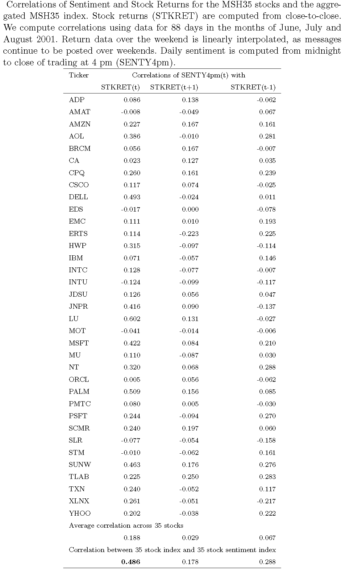
7.35.3 Phase Lag Analysis
7.36 False Positives
The percentage of false positives is a useful metric to work with. It may be calculated as a simple count or as a weighted count (by nearness of wrong category) of false classifications divided by total classifications undertaken.
For example, assume that in the example above, category 1 is BULLISH and category 3 is BEARISH, whereas category 2 is NEUTRAL. The false positives would arise from mis-classifying category 1 as 3 and vice-versa. We compute the false positive rate for illustration.
The false positive rate is just 1% in the example below.
Omatrix = matrix(c(22,1,0,3,44,3,1,1,25),3,3)
print((Omatrix[1,3]+Omatrix[3,1])/sum(Omatrix))
## [1] 0.017.37 Sentiment Error
In a 3-way classification scheme, where category 1 is BULLISH and category 3 is BEARISH, whereas category 2 is NEUTRAL, we can compute this metric as follows.
\[ \mbox{Sentiment Error} = 1 - \frac{M(j=1)-M(j=3)}{M(i=1)-M(i=3)} \nonumber \]
In our illustrative example, we may easily calculate this metric. The classified sentiment from the algorithm was \(-3 = 23-27\), whereas it actually should have been \(-2 = 26-28\). The percentage error in sentiment is 50%.
print(Omatrix)## [,1] [,2] [,3]
## [1,] 22 3 1
## [2,] 1 44 1
## [3,] 0 3 25rsum = rowSums(Omatrix)
csum = colSums(Omatrix)
print(rsum)## [1] 26 46 28print(csum)## [1] 23 50 27print(1 - (-3)/(-2))## [1] -0.57.38 Disagreement
The metric uses the number of signed buys and sells in the day (based on a sentiment model) to determine how much difference of opinion there is in the market. The metric is computed as follows:
\[ \mbox{DISAG} = \left| 1 - \left| \frac{B-S}{B+S} \right| \right| \]
where \(B, S\) are the numbers of classified buys and sells. Note that DISAG is bounded between zero and one.
Using the true categories of buys (category 1 BULLISH) and sells (category 3 BEARISH) in the same example as before, we may compute disagreement. Since there is little agreement (26 buys and 28 sells), disagreement is high.
print(Omatrix)## [,1] [,2] [,3]
## [1,] 22 3 1
## [2,] 1 44 1
## [3,] 0 3 25DISAG = abs(1-abs((26-28)/(26+28)))
print(DISAG)## [1] 0.9629637.39 Precision and Recall
The creation of the confusion matrix leads naturally to two measures that are associated with it.
Precision is the fraction of positives identified that are truly positive, and is also known as positive predictive value. It is a measure of usefulness of prediction. So if the algorithm (say) was tasked with selecting those account holders on LinkedIn who are actually looking for a job, and it identifies \(n\) such people of which only \(m\) were really looking for a job, then the precision would be \(m/n\).
Recall is the proportion of positives that are correctly identified, and is also known as sensitivity. It is a measure of how complete the prediction is. If the actual number of people looking for a job on LinkedIn was \(M\), then recall would be \(n/M\).
For example, suppose we have the following confusion matrix.
| Actual | |||
|---|---|---|---|
| Predicted | Looking for Job | Not Looking | |
| Looking for Job | 10 | 2 | 12 |
| Not Looking | 1 | 16 | 17 |
| 11 | 18 | 29 |
In this case precision is \(10/12\) and recall is \(10/11\). Precision is related to the probability of false positives (Type I error), which is one minus precision. Recall is related to the probability of false negatives (Type II error), which is one minus recall.
One may also think of this in terms of true and false positives. There are totally 12 positives predicted by the model, of which 10 are true positives, and 2 are false positives. These values go into calculating precision.
Of the predicted negatives, 1 is false, and this goes into calculating recall. Recall refers to relevancy of results returned.
7.40 RTextTools package
This package bundles text classification algorithms into one package.
library(tm)
library(RTextTools)
## Loading required package: SparseM## Warning: package 'SparseM' was built under R version 3.3.2##
## Attaching package: 'SparseM'## The following object is masked from 'package:base':
##
## backsolve##
## Attaching package: 'RTextTools'## The following objects are masked from 'package:SnowballC':
##
## getStemLanguages, wordStem#Create sample text with positive and negative markers
n = 1000
npos = round(runif(n,1,25))
nneg = round(runif(n,1,25))
flag = matrix(0,n,1)
flag[which(npos>nneg)] = 1
text = NULL
for (j in 1:n) {
res = paste(c(sample(poswords,npos[j]),sample(negwords,nneg[j])),collapse=" ")
text = c(text,res)
}
#Text Classification
m = create_matrix(text)
print(m)## <<DocumentTermMatrix (documents: 1000, terms: 3711)>>
## Non-/sparse entries: 26023/3684977
## Sparsity : 99%
## Maximal term length: 17
## Weighting : term frequency (tf)m = create_matrix(text,weighting=weightTfIdf)
print(m)## <<DocumentTermMatrix (documents: 1000, terms: 3711)>>
## Non-/sparse entries: 26023/3684977
## Sparsity : 99%
## Maximal term length: 17
## Weighting : term frequency - inverse document frequency (normalized) (tf-idf)container <- create_container(m,flag,trainSize=1:(n/2), testSize=(n/2+1):n,virgin=FALSE)
#models <- train_models(container, algorithms=c("MAXENT","SVM","GLMNET","SLDA","TREE","BAGGING","BOOSTING","RF"))
models <- train_models(container, algorithms=c("MAXENT","SVM","GLMNET","TREE"))
results <- classify_models(container, models)
analytics <- create_analytics(container, results)
#RESULTS
#analytics@algorithm_summary # SUMMARY OF PRECISION, RECALL, F-SCORES, AND ACCURACY SORTED BY TOPIC CODE FOR EACH ALGORITHM
#analytics@label_summary # SUMMARY OF LABEL (e.g. TOPIC) ACCURACY
#analytics@document_summary # RAW SUMMARY OF ALL DATA AND SCORING
#analytics@ensemble_summary # SUMMARY OF ENSEMBLE PRECISION/COVERAGE. USES THE n VARIABLE PASSED INTO create_analytics()
#CONFUSION MATRIX
yhat = as.matrix(analytics@document_summary$CONSENSUS_CODE)
y = flag[(n/2+1):n]
print(table(y,yhat))## yhat
## y 0 1
## 0 255 6
## 1 212 277.41 Grading Text
In recent years, the SAT exams added a new essay section. While the test aimed at assessing original writing, it also introduced automated grading. A goal of the test is to assess the writing level of the student. This is associated with the notion of readability.
7.41.1 Readability
“Readability” is a metric of how easy it is to comprehend text. Given a goal of efficient markets, regulators want to foster transparency by making sure financial documents that are disseminated to the investing public are readable. Hence, metrics for readability are very important and are recently gaining traction.
7.41.2 Gunning-Fog Index
Gunning (1952) developed the Fog index. The index estimates the years of formal education needed to understand text on a first reading. A fog index of 12 requires the reading level of a U.S. high school senior (around 18 years old). The index is based on the idea that poor readability is associated with longer sentences and complex words. Complex words are those that have more than two syllables. The formula for the Fog index is
\[ 0.4 \cdot \left[\frac{\mbox{\#words}}{\mbox{\#sentences}} + 100 \cdot \left( \frac{\mbox{\#complex words}}{\mbox{\#words}} \right) \right] \]
Alternative readability scores use similar ideas. The Flesch Reading Ease Score and the Flesch-Kincaid Grade Level also use counts of words, syllables, and sentences. See http://en.wikipedia.org/wiki/Flesch-Kincaid_readability_tests. The Flesch Reading Ease Score is defined as
\[ 206.835 - 1.015 \left(\frac{\mbox{\#words}}{\mbox{\#sentences}}\right) - 84.6 \left( \frac{\mbox{\#syllables}}{\mbox{\#words}} \right) \]
With a range of 90-100 easily accessible by a 11-year old, 60-70 being easy to understand for 13-15 year olds, and 0-30 for university graduates.
7.41.3 The Flesch-Kincaid Grade Level
This is defined as
\[ 0.39 \left(\frac{\mbox{\#words}}{\mbox{\#sentences}}\right) + 11.8 \left( \frac{\mbox{\#syllables}}{\mbox{\#words}} \right) -15.59 \]
which gives a number that corresponds to the grade level. As expected these two measures are negatively correlated. Various other measures of readability use the same ideas as in the Fog index. For example the Coleman and Liau (1975) index does not even require a count of syllables, as follows:
\[ CLI = 0.0588 L - 0.296 S - 15.8 \]
where \(L\) is the average number of letters per hundred words and \(S\) is the average number of sentences per hundred words.
Standard readability metrics may not work well for financial text. Loughran and McDonald (2014) find that the Fog index is inferior to simply looking at 10-K file size.
References
M. Coleman and T. L. Liau. (1975). A computer readability formula designed for machine scoring. Journal of Applied Psychology 60, 283-284.
T. Loughran and W. McDonald, (2014). Measuring readability in financial disclosures, The Journal of Finance 69, 1643-1671.
7.42 koRpus package
R package koRpus for readability scoring here. http://www.inside-r.org/packages/cran/koRpus/docs/readability
First, let’s grab some text from my web site.
library(rvest)
url = "http://srdas.github.io/bio-candid.html"

doc.html = read_html(url)
text = doc.html %>% html_nodes("p") %>% html_text()

text = gsub("[\t\n]"," ",text)
text = gsub('"'," ",text)   #removes single backslash
text = paste(text, collapse=" ")
print(text)
## [1] " Sanjiv Das: A Short Academic Life History After loafing and working in many parts of Asia, but never really growing up, Sanjiv moved to New York to change the world, hopefully through research. He graduated in 1994 with a Ph.D. from NYU, and since then spent five years in Boston, and now lives in San Jose, California. Sanjiv loves animals, places in the world where the mountains meet the sea, riding sport motorbikes, reading, gadgets, science fiction movies, and writing cool software code. When there is time available from the excitement of daily life, Sanjiv writes academic papers, which helps him relax. Always the contrarian, Sanjiv thinks that New York City is the most calming place in the world, after California of course. Sanjiv is now a Professor of Finance at Santa Clara University. He came to SCU from Harvard Business School and spent a year at UC Berkeley. In his past life in the unreal world, Sanjiv worked at Citibank, N.A. in the Asia-Pacific region. He takes great pleasure in merging his many previous lives into his current existence, which is incredibly confused and diverse. Sanjiv's research style is instilled with a distinct New York state of mind - it is chaotic, diverse, with minimal method to the madness. He has published articles on derivatives, term-structure models, mutual funds, the internet, portfolio choice, banking models, credit risk, and has unpublished articles in many other areas. Some years ago, he took time off to get another degree in computer science at Berkeley, confirming that an unchecked hobby can quickly become an obsession. There he learnt about the fascinating field of Randomized Algorithms, skills he now applies earnestly to his editorial work, and other pursuits, many of which stem from being in the epicenter of Silicon Valley. Coastal living did a lot to mold Sanjiv, who needs to live near the ocean. The many walks in Greenwich village convinced him that there is no such thing as a representative investor, yet added many unique features to his personal utility function. He learnt that it is important to open the academic door to the ivory tower and let the world in. Academia is a real challenge, given that he has to reconcile many more opinions than ideas. He has been known to have turned down many offers from Mad magazine to publish his academic work. As he often explains, you never really finish your education - you can check out any time you like, but you can never leave. Which is why he is doomed to a lifetime in Hotel California. And he believes that, if this is as bad as it gets, life is really pretty good. "Now we can assess it for readability.
library(koRpus)##
## Attaching package: 'koRpus'## The following object is masked from 'package:lsa':
##
## querywrite(text,file="textvec.txt")
text_tokens = tokenize("textvec.txt",lang="en")
#print(text_tokens)
print(c("Number of sentences: ",text_tokens@desc$sentences))## [1] "Number of sentences: " "24"print(c("Number of words: ",text_tokens@desc$words))## [1] "Number of words: " "446"print(c("Number of words per sentence: ",text_tokens@desc$avg.sentc.length))## [1] "Number of words per sentence: " "18.5833333333333"print(c("Average length of words: ",text_tokens@desc$avg.word.length))## [1] "Average length of words: " "4.67488789237668"Next we generate several indices of readability, which are worth looking at.
print(readability(text_tokens))## Hyphenation (language: en)##
|
| | 0%
|
| | 1%
|
|= | 1%
|
|= | 2%
|
|== | 2%
|
|== | 3%
|
|== | 4%
|
|=== | 4%
|
|=== | 5%
|
|==== | 6%
|
|==== | 7%
|
|===== | 7%
|
|===== | 8%
|
|====== | 9%
|
|====== | 10%
|
|======= | 10%
|
|======= | 11%
|
|======== | 12%
|
|======== | 13%
|
|========= | 13%
|
|========= | 14%
|
|========= | 15%
|
|========== | 15%
|
|========== | 16%
|
|=========== | 16%
|
|=========== | 17%
|
|============ | 18%
|
|============ | 19%
|
|============= | 19%
|
|============= | 20%
|
|============= | 21%
|
|============== | 21%
|
|============== | 22%
|
|=============== | 22%
|
|=============== | 23%
|
|=============== | 24%
|
|================ | 24%
|
|================ | 25%
|
|================= | 26%
|
|================= | 27%
|
|================== | 27%
|
|================== | 28%
|
|=================== | 28%
|
|=================== | 29%
|
|=================== | 30%
|
|==================== | 30%
|
|==================== | 31%
|
|===================== | 32%
|
|===================== | 33%
|
|====================== | 33%
|
|====================== | 34%
|
|====================== | 35%
|
|======================= | 35%
|
|======================= | 36%
|
|======================== | 36%
|
|======================== | 37%
|
|======================== | 38%
|
|========================= | 38%
|
|========================= | 39%
|
|========================== | 39%
|
|========================== | 40%
|
|========================== | 41%
|
|=========================== | 41%
|
|=========================== | 42%
|
|============================ | 42%
|
|============================ | 43%
|
|============================ | 44%
|
|============================= | 44%
|
|============================= | 45%
|
|============================== | 46%
|
|============================== | 47%
|
|=============================== | 47%
|
|=============================== | 48%
|
|================================ | 49%
|
|================================ | 50%
|
|================================= | 50%
|
|================================= | 51%
|
|================================== | 52%
|
|================================== | 53%
|
|=================================== | 53%
|
|=================================== | 54%
|
|==================================== | 55%
|
|==================================== | 56%
|
|===================================== | 56%
|
|===================================== | 57%
|
|===================================== | 58%
|
|====================================== | 58%
|
|====================================== | 59%
|
|======================================= | 59%
|
|======================================= | 60%
|
|======================================= | 61%
|
|======================================== | 61%
|
|======================================== | 62%
|
|========================================= | 62%
|
|========================================= | 63%
|
|========================================= | 64%
|
|========================================== | 64%
|
|========================================== | 65%
|
|=========================================== | 65%
|
|=========================================== | 66%
|
|=========================================== | 67%
|
|============================================ | 67%
|
|============================================ | 68%
|
|============================================= | 69%
|
|============================================= | 70%
|
|============================================== | 70%
|
|============================================== | 71%
|
|============================================== | 72%
|
|=============================================== | 72%
|
|=============================================== | 73%
|
|================================================ | 73%
|
|================================================ | 74%
|
|================================================= | 75%
|
|================================================= | 76%
|
|================================================== | 76%
|
|================================================== | 77%
|
|================================================== | 78%
|
|=================================================== | 78%
|
|=================================================== | 79%
|
|==================================================== | 79%
|
|==================================================== | 80%
|
|==================================================== | 81%
|
|===================================================== | 81%
|
|===================================================== | 82%
|
|====================================================== | 83%
|
|====================================================== | 84%
|
|======================================================= | 84%
|
|======================================================= | 85%
|
|======================================================== | 85%
|
|======================================================== | 86%
|
|======================================================== | 87%
|
|========================================================= | 87%
|
|========================================================= | 88%
|
|========================================================== | 89%
|
|========================================================== | 90%
|
|=========================================================== | 90%
|
|=========================================================== | 91%
|
|============================================================ | 92%
|
|============================================================ | 93%
|
|============================================================= | 93%
|
|============================================================= | 94%
|
|============================================================== | 95%
|
|============================================================== | 96%
|
|=============================================================== | 96%
|
|=============================================================== | 97%
|
|=============================================================== | 98%
|
|================================================================ | 98%
|
|================================================================ | 99%
|
|=================================================================| 99%
|
|=================================================================| 100%## Warning: Bormuth: Missing word list, hence not calculated.## Warning: Coleman: POS tags are not elaborate enough, can't count pronouns
## and prepositions. Formulae skipped.## Warning: Dale-Chall: Missing word list, hence not calculated.## Warning: DRP: Missing Bormuth Mean Cloze, hence not calculated.## Warning: Harris.Jacobson: Missing word list, hence not calculated.## Warning: Spache: Missing word list, hence not calculated.## Warning: Traenkle.Bailer: POS tags are not elaborate enough, can't count
## prepositions and conjuctions. Formulae skipped.## Warning: Note: The implementations of these formulas are still subject to validation:
## Coleman, Danielson.Bryan, Dickes.Steiwer, ELF, Fucks, Harris.Jacobson, nWS, Strain, Traenkle.Bailer, TRI
## Use the results with caution, even if they seem plausible!##
## Automated Readability Index (ARI)
## Parameters: default
## Grade: 9.88
##
##
## Coleman-Liau
## Parameters: default
## ECP: 47% (estimted cloze percentage)
## Grade: 10.09
## Grade: 10.1 (short formula)
##
##
## Danielson-Bryan
## Parameters: default
## DB1: 7.64
## DB2: 48.58
## Grade: 9-12
##
##
## Dickes-Steiwer's Handformel
## Parameters: default
## TTR: 0.58
## Score: 42.76
##
##
## Easy Listening Formula
## Parameters: default
## Exsyls: 149
## Score: 6.21
##
##
## Farr-Jenkins-Paterson
## Parameters: default
## RE: 56.1
## Grade: >= 10 (high school)
##
##
## Flesch Reading Ease
## Parameters: en (Flesch)
## RE: 59.75
## Grade: >= 10 (high school)
##
##
## Flesch-Kincaid Grade Level
## Parameters: default
## Grade: 9.54
## Age: 14.54
##
##
## Gunning Frequency of Gobbledygook (FOG)
## Parameters: default
## Grade: 12.55
##
##
## FORCAST
## Parameters: default
## Grade: 10.01
## Age: 15.01
##
##
## Fucks' Stilcharakteristik
## Score: 86.88
## Grade: 9.32
##
##
## Linsear Write
## Parameters: default
## Easy words: 87
## Hard words: 13
## Grade: 11.71
##
##
## Läsbarhetsindex (LIX)
## Parameters: default
## Index: 40.56
## Rating: standard
## Grade: 6
##
##
## Neue Wiener Sachtextformeln
## Parameters: default
## nWS 1: 5.42
## nWS 2: 5.97
## nWS 3: 6.28
## nWS 4: 6.81
##
##
## Readability Index (RIX)
## Parameters: default
## Index: 4.08
## Grade: 9
##
##
## Simple Measure of Gobbledygook (SMOG)
## Parameters: default
## Grade: 12.01
## Age: 17.01
##
##
## Strain Index
## Parameters: default
## Index: 8.45
##
##
## Kuntzsch's Text-Redundanz-Index
## Parameters: default
## Short words: 297
## Punctuation: 71
## Foreign: 0
## Score: -56.22
##
##
## Tuldava's Text Difficulty Formula
## Parameters: default
## Index: 4.43
##
##
## Wheeler-Smith
## Parameters: default
## Score: 62.08
## Grade: > 4
##
## Text language: en7.43 Text Summarization
It is really easy to write a summarizer in a few lines of code. The function below takes in a text array and does the needful. Each element of the array is one sentence of the document we wan summarized.
In the function we need to calculate how similar each sentence is to any other one. This could be done using cosine similarity, but here we use another approach, Jaccard similarity. Given two sentences, Jaccard similarity is the ratio of the size of the intersection word set divided by the size of the union set.
7.43.1 Jaccard Similarity
A document \(D\) is comprised of \(m\) sentences \(s_i, i=1,2,...,m\), where each \(s_i\) is a set of words. We compute the pairwise overlap between sentences using the Jaccard similarity index:
\[ J_{ij} = J(s_i, s_j) = \frac{|s_i \cap s_j|}{|s_i \cup s_j|} = J_{ji} \]
The overlap is the ratio of the size of the intersect of the two word sets in sentences \(s_i\) and \(s_j\), divided by the size of the union of the two sets. The similarity score of each sentence is computed as the row sums of the Jaccard similarity matrix.
\[ {\cal S}_i = \sum_{j=1}^m J_{ij} \]
7.43.2 Generating the summary
Once the row sums are obtained, they are sorted and the summary is the first \(n\) sentences based on the \({\cal S}_i\) values.
# FUNCTION TO RETURN n SENTENCE SUMMARY
# Input: array of sentences (text)
# Output: n most common intersecting sentences
text_summary = function(text, n) {
m = length(text) # No of sentences in input
jaccard = matrix(0,m,m) #Store match index
for (i in 1:m) {
for (j in i:m) {
a = text[i]; aa = unlist(strsplit(a," "))
b = text[j]; bb = unlist(strsplit(b," "))
jaccard[i,j] = length(intersect(aa,bb))/
length(union(aa,bb))
jaccard[j,i] = jaccard[i,j]
}
}
similarity_score = rowSums(jaccard)
res = sort(similarity_score, index.return=TRUE,
decreasing=TRUE)
idx = res$ix[1:n]
summary = text[idx]
}7.43.3 Example: Summarization
We will use a sample of text that I took from Bloomberg news. It is about the need for data scientists.
url = "DSTMAA_data/dstext_sample.txt" #You can put any text file or URL here
text = read_web_page(url,cstem=0,cstop=0,ccase=0,cpunc=0,cflat=1)
print(length(text[[1]]))## [1] 1print("ORIGINAL TEXT")## [1] "ORIGINAL TEXT"print(text)## [1] "THERE HAVE BEEN murmurings that we are now in the “trough of disillusionment” of big data, the hype around it having surpassed the reality of what it can deliver. Gartner suggested that the “gravitational pull of big data is now so strong that even people who haven’t a clue as to what it’s all about report that they’re running big data projects.” Indeed, their research with business decision makers suggests that organisations are struggling to get value from big data. Data scientists were meant to be the answer to this issue. Indeed, Hal Varian, Chief Economist at Google famously joked that “The sexy job in the next 10 years will be statisticians.” He was clearly right as we are now used to hearing that data scientists are the key to unlocking the value of big data. This has created a huge market for people with these skills. US recruitment agency, Glassdoor, report that the average salary for a data scientist is $118,709 versus $64,537 for a skilled programmer. And a McKinsey study predicts that by 2018, the United States alone faces a shortage of 140,000 to 190,000 people with analytical expertise and a 1.5 million shortage of managers with the skills to understand and make decisions based on analysis of big data. It’s no wonder that companies are keen to employ data scientists when, for example, a retailer using big data can reportedly increase their margin by more than 60%. However, is it really this simple? Can data scientists actually justify earning their salaries when brands seem to be struggling to realize the promise of big data? Perhaps we are expecting too much of data scientists. May be we are investing too much in a relatively small number of individuals rather than thinking about how we can design organisations to help us get the most from data assets. The focus on the data scientist often implies a centralized approach to analytics and decision making; we implicitly assume that a small team of highly skilled individuals can meet the needs of the organisation as a whole. This theme of centralized vs. decentralized decision-making is one that has long been debated in the management literature. For many organisations a centralized structure helps maintain control over a vast international operation, plus ensures consistency of customer experience. Others, meanwhile, may give managers at a local level decision-making power particularly when it comes to tactical needs. But the issue urgently needs revisiting in the context of big data as the way in which organisations manage themselves around data may well be a key factor for brands in realizing the value of their data assets. Economist and philosopher Friedrich Hayek took the view that organisations should consider the purpose of the information itself. Centralized decision-making can be more cost-effective and co-ordinated, he believed, but decentralization can add speed and local information that proves more valuable, even if the bigger picture is less clear. He argued that organisations thought too highly of centralized knowledge, while ignoring ‘knowledge of the particular circumstances of time and place’. But it is only relatively recently that economists are starting to accumulate data that allows them to gauge how successful organisations organize themselves. One such exercise reported by Tim Harford was carried out by Harvard Professor Julie Wulf and the former chief economist of the International Monetary Fund, Raghuram Rajan. They reviewed the workings of large US organisations over fifteen years from the mid-80s. What they found was successful companies were often associated with a move towards decentralisation, often driven by globalisation and the need to react promptly to a diverse and swiftly-moving range of markets, particularly at a local level. Their research indicated that decentralisation pays. And technological advancement often goes hand-in-hand with decentralization. Data analytics is starting to filter down to the department layer, where executives are increasingly eager to trawl through the mass of information on offer. Cloud computing, meanwhile, means that line managers no longer rely on IT teams to deploy computer resources. They can do it themselves, in just minutes. The decentralization trend is now impacting on technology spending. According to Gartner, chief marketing officers have been given the same purchasing power in this area as IT managers and, as their spending rises, so that of data centre managers is falling. Tim Harford makes a strong case for the way in which this decentralization is important given that the environment in which we operate is so unpredictable. Innovation typically comes, he argues from a “swirling mix of ideas not from isolated minds.” And he cites Jane Jacobs, writer on urban planning– who suggested we find innovation in cities rather than on the Pacific islands. But this approach is not necessarily always adopted. For example, research by academics Donald Marchand and Joe Peppard discovered that there was still a tendency for brands to approach big data projects the same way they would existing IT projects: i.e. using centralized IT specialists with a focus on building and deploying technology on time, to plan, and within budget. The problem with a centralized ‘IT-style’ approach is that it ignores the human side of the process of considering how people create and use information i.e. how do people actually deliver value from data assets. Marchand and Peppard suggest (among other recommendations) that those who need to be able to create meaning from data should be at the heart of any initiative. As ever then, the real value from data comes from asking the right questions of the data. And the right questions to ask only emerge if you are close enough to the business to see them. Are data scientists earning their salary? In my view they are a necessary but not sufficient part of the solution; brands need to be making greater investment in working with a greater range of users to help them ask questions of the data. Which probably means that data scientists’ salaries will need to take a hit in the process."text2 = strsplit(text,". ",fixed=TRUE) #Special handling of the period.
text2 = text2[[1]]
print("SENTENCES")## [1] "SENTENCES"print(text2)## [1] "THERE HAVE BEEN murmurings that we are now in the “trough of disillusionment” of big data, the hype around it having surpassed the reality of what it can deliver"
## [2] " Gartner suggested that the “gravitational pull of big data is now so strong that even people who haven’t a clue as to what it’s all about report that they’re running big data projects.” Indeed, their research with business decision makers suggests that organisations are struggling to get value from big data"
## [3] "Data scientists were meant to be the answer to this issue"
## [4] "Indeed, Hal Varian, Chief Economist at Google famously joked that “The sexy job in the next 10 years will be statisticians.” He was clearly right as we are now used to hearing that data scientists are the key to unlocking the value of big data"
## [5] "This has created a huge market for people with these skills"
## [6] "US recruitment agency, Glassdoor, report that the average salary for a data scientist is $118,709 versus $64,537 for a skilled programmer"
## [7] "And a McKinsey study predicts that by 2018, the United States alone faces a shortage of 140,000 to 190,000 people with analytical expertise and a 1.5 million shortage of managers with the skills to understand and make decisions based on analysis of big data"
## [8] " It’s no wonder that companies are keen to employ data scientists when, for example, a retailer using big data can reportedly increase their margin by more than 60%"
## [9] " However, is it really this simple? Can data scientists actually justify earning their salaries when brands seem to be struggling to realize the promise of big data? Perhaps we are expecting too much of data scientists"
## [10] "May be we are investing too much in a relatively small number of individuals rather than thinking about how we can design organisations to help us get the most from data assets"
## [11] "The focus on the data scientist often implies a centralized approach to analytics and decision making; we implicitly assume that a small team of highly skilled individuals can meet the needs of the organisation as a whole"
## [12] "This theme of centralized vs"
## [13] "decentralized decision-making is one that has long been debated in the management literature"
## [14] " For many organisations a centralized structure helps maintain control over a vast international operation, plus ensures consistency of customer experience"
## [15] "Others, meanwhile, may give managers at a local level decision-making power particularly when it comes to tactical needs"
## [16] " But the issue urgently needs revisiting in the context of big data as the way in which organisations manage themselves around data may well be a key factor for brands in realizing the value of their data assets"
## [17] "Economist and philosopher Friedrich Hayek took the view that organisations should consider the purpose of the information itself"
## [18] "Centralized decision-making can be more cost-effective and co-ordinated, he believed, but decentralization can add speed and local information that proves more valuable, even if the bigger picture is less clear"
## [19] " He argued that organisations thought too highly of centralized knowledge, while ignoring ‘knowledge of the particular circumstances of time and place’"
## [20] "But it is only relatively recently that economists are starting to accumulate data that allows them to gauge how successful organisations organize themselves"
## [21] "One such exercise reported by Tim Harford was carried out by Harvard Professor Julie Wulf and the former chief economist of the International Monetary Fund, Raghuram Rajan"
## [22] "They reviewed the workings of large US organisations over fifteen years from the mid-80s"
## [23] "What they found was successful companies were often associated with a move towards decentralisation, often driven by globalisation and the need to react promptly to a diverse and swiftly-moving range of markets, particularly at a local level"
## [24] "Their research indicated that decentralisation pays"
## [25] "And technological advancement often goes hand-in-hand with decentralization"
## [26] "Data analytics is starting to filter down to the department layer, where executives are increasingly eager to trawl through the mass of information on offer"
## [27] "Cloud computing, meanwhile, means that line managers no longer rely on IT teams to deploy computer resources"
## [28] "They can do it themselves, in just minutes"
## [29] " The decentralization trend is now impacting on technology spending"
## [30] "According to Gartner, chief marketing officers have been given the same purchasing power in this area as IT managers and, as their spending rises, so that of data centre managers is falling"
## [31] "Tim Harford makes a strong case for the way in which this decentralization is important given that the environment in which we operate is so unpredictable"
## [32] "Innovation typically comes, he argues from a “swirling mix of ideas not from isolated minds.” And he cites Jane Jacobs, writer on urban planning– who suggested we find innovation in cities rather than on the Pacific islands"
## [33] "But this approach is not necessarily always adopted"
## [34] "For example, research by academics Donald Marchand and Joe Peppard discovered that there was still a tendency for brands to approach big data projects the same way they would existing IT projects: i.e"
## [35] "using centralized IT specialists with a focus on building and deploying technology on time, to plan, and within budget"
## [36] "The problem with a centralized ‘IT-style’ approach is that it ignores the human side of the process of considering how people create and use information i.e"
## [37] "how do people actually deliver value from data assets"
## [38] "Marchand and Peppard suggest (among other recommendations) that those who need to be able to create meaning from data should be at the heart of any initiative"
## [39] "As ever then, the real value from data comes from asking the right questions of the data"
## [40] "And the right questions to ask only emerge if you are close enough to the business to see them"
## [41] "Are data scientists earning their salary? In my view they are a necessary but not sufficient part of the solution; brands need to be making greater investment in working with a greater range of users to help them ask questions of the data"
## [42] "Which probably means that data scientists’ salaries will need to take a hit in the process."print("SUMMARY")## [1] "SUMMARY"res = text_summary(text2,5)
print(res)## [1] " Gartner suggested that the “gravitational pull of big data is now so strong that even people who haven’t a clue as to what it’s all about report that they’re running big data projects.” Indeed, their research with business decision makers suggests that organisations are struggling to get value from big data"
## [2] "The focus on the data scientist often implies a centralized approach to analytics and decision making; we implicitly assume that a small team of highly skilled individuals can meet the needs of the organisation as a whole"
## [3] "May be we are investing too much in a relatively small number of individuals rather than thinking about how we can design organisations to help us get the most from data assets"
## [4] "The problem with a centralized ‘IT-style’ approach is that it ignores the human side of the process of considering how people create and use information i.e"
## [5] "Which probably means that data scientists’ salaries will need to take a hit in the process."7.44 Research in Finance
In this segment we explore various text mining research in the field of finance.
Lu, Chen, Chen, Hung, and Li (2010) categorize finance related textual content into three categories: (a) forums, blogs, and wikis; (b) news and research reports; and (c) content generated by firms.
Extracting sentiment and other information from messages posted to stock message boards such as Yahoo!, Motley Fool, Silicon Investor, Raging Bull, etc., see Tumarkin and Whitelaw (2001), Antweiler and Frank (2004), Antweiler and Frank (2005), Das, Martinez-Jerez and Tufano (2005), Das and Chen (2007).
Other news sources: Lexis-Nexis, Factiva, Dow Jones News, etc., see Das, Martinez-Jerez and Tufano (2005); Boudoukh, Feldman, Kogan, Richardson (2012).
The Heard on the Street column in the Wall Street Journal has been used in work by Tetlock (2007), Tetlock, Saar-Tsechansky and Macskassay (2008); see also the use of Wall Street Journal articles by Lu, Chen, Chen, Hung, and Li (2010).
Thomson-Reuters NewsScope Sentiment Engine (RNSE) based on Infonics/Lexalytics algorithms and varied data on stocks and text from internal databases, see Leinweber and Sisk (2011). Zhang and Skiena (2010) develop a market neutral trading strategy using news media such as tweets, over 500 newspapers, Spinn3r RSS feeds, and LiveJournal.
7.44.1 Das and Chen (Management Science 2007)

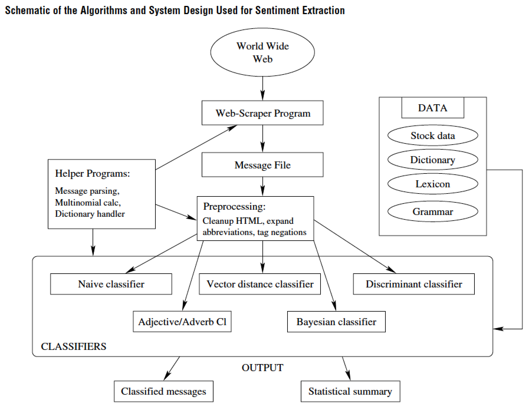
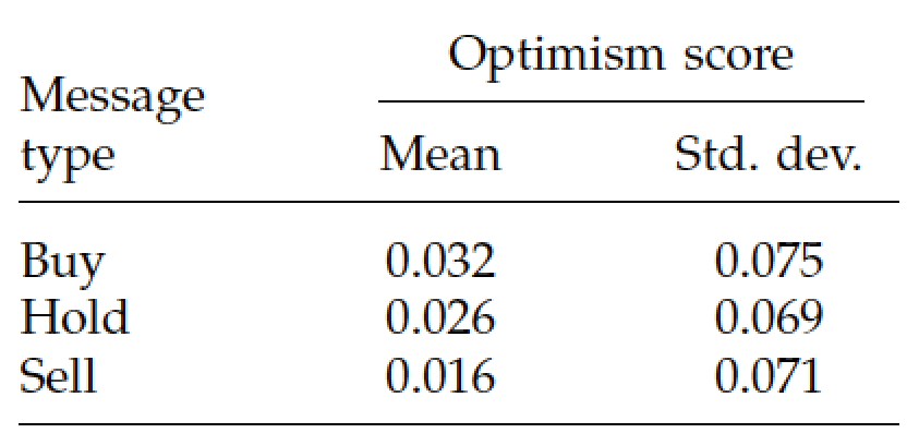
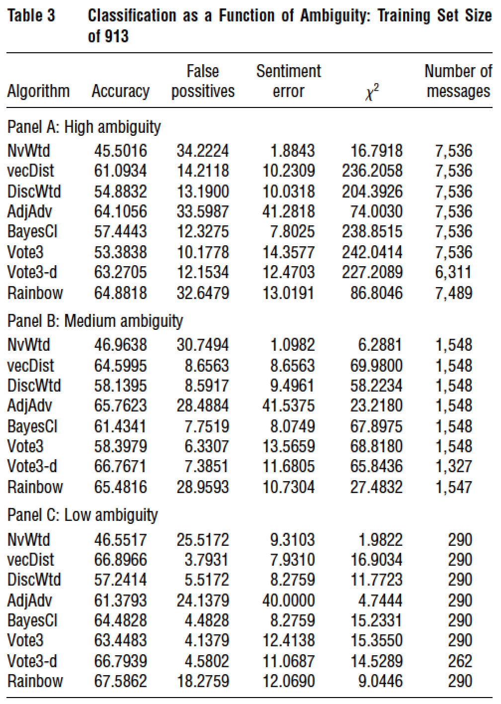
7.44.2 Using Twitter and Facebook for Market Prediction
Bollen, Mao, and Zeng (2010) claimed that stock direction of the Dow Jones Industrial Average can be predicted using tweets with 87.6% accuracy.
Bar-Haim, Dinur, Feldman, Fresko and Goldstein (2011) attempt to predict stock direction using tweets by detecting and overweighting the opinion of expert investors.
Brown (2012) looks at the correlation between tweets and the stock market via several measures.
Logunov (2011) uses OpinionFinder to generate many measures of sentiment from tweets.
Twitter based sentiment developed by Rao and Srivastava (2012) is found to be highly correlated with stock prices and indexes, as high as 0.88 for returns.
Sprenger and Welpe (2010) find that tweet bullishness is associated with abnormal stock returns and tweet volume predicts trading volume.
7.45 Polarity and Subjectivity
Zhang and Skiena (2010) use Twitter feeds and also three other sources of text: over 500 nationwide newspapers, RSS feeds from blogs, and LiveJournal blogs. These are used to compute two metrics.
\[ \mbox{polarity} = \frac{n_{pos} - n_{neg}}{n_{pos} + n_{neg}} \]
\[ \mbox{subjectivity} = \frac{n_{pos} + n_{neg}}{N} \]
where \(N\) is the total number of words in a text document, \(n_{pos}, n_{neg}\) are the number of positive and negative words, respectively.
They find that the number of articles is predictive of trading volume.
Subjectivity is also predictive of trading volume, lending credence to the idea that differences of opinion make markets.
Stock return prediction is weak using polarity, but tweets do seem to have some predictive power.
Various sentiment driven market neutral strategies are shown to be profitable, though the study is not tested for robustness.
Logunov (2011) uses tweets data, and applies OpinionFinder and also developed a new classifier called Naive Emoticon Classification to encode sentiment. This is an unusual and original, albeit quite intuitive use of emoticons to determine mood in text mining. If an emoticon exists, then the tweet is automatically coded with that sentiment of emotion. Four types of emoticons are considered: Happy (H), Sad (S), Joy (J), and Cry (C). Polarity is defined here as
\[ \mbox{polarity} = A = \frac{n_H + n_J}{n_H + n_S + n_J + n_C} \]
Values greater than 0.5 are positive. \(A\) stands for aggregate sentiment and appears to be strongly autocorrelated. Overall, prediction evidence is weak.
7.45.1 Text Mining Corporate Reports
Text analysis is undertaken across companies in a cross-section.
The quality of text in company reports is much better than in message postings.
Textual analysis in this area has also resulted in technical improvements. Rudimentary approaches such as word count methods have been extended to weighted schemes, where weights are determined in statistical ways. In Das and Chen (2007), the discriminant score of each word across classification categories is used as a weighting index for the importance of words.
There is a proliferation of word-weighting schemes.The idea of “inverse document frequency’’ (\(idf\)) as a weighting coefficient. Hence, the \(idf\) for word \(j\) would be
\[ w_j^{idf} = \ln \left( \frac{N}{df_j} \right) \] where \(N\) is the total number of documents, and \(df_j\) is the number of documents containing word \(j\). This scheme was proposed by Manning and Schutze (1999).
- Loughran and McDonald (2011) use this weighting approach to modify the word (term) frequency counts in the documents they analyze. The weight on word \(j\) in document \(i\) is specified as
\[ w_{ij} = \max[0,1 + \ln(f_{ij}) w_{j}^{idf}] \]
where \(f_{ij}\) is the frequency count of word \(j\) in document \(i\). This leads naturally to a document score of
\[ S_i^{LM} = \frac{1}{1+\ln(a_i)} \sum_{j=1}^J w_{ij} \]
Here \(a_i\) is the total number of words in document \(i\), and \(J\) is the total number of words in the lexicon. (The \(LM\) superscript signifies the weighting approach.)
Whereas the \(idf\) approach is intuitive, it does not have to be relevant for market activity. An alternate and effective weighting scheme has been developed in Jegadeesh and Wu (2013, JW) using market movements. Words that occur more often on large market move days are given a greater weight than other words. JW show that this scheme is superior to an unweighted one, and delivers an accurate system for determining the “tone’’ of a regulatory filing.
JW also conduct robustness checks that suggest that the approach is quite general, and applies to other domains with no additional modifications to the specification. Indeed, they find that tone extraction from 10-Ks may be used to predict IPO underpricing.
7.46 Tone
Jegadeesh and Wu (2013) create a “global lexicon’’ merging multiple word lists from Harvard-IV-4 Psychological Dictionaries(Harvard Inquirer), the Lasswell Value Dictionary, the Loughran and McDonald lists, and the word list in Bradley and Lang (1999). They test this lexicon for robustness by checking (a) that the lexicon delivers accurate tone scores and (b) that it is complete by discarding 50% of the words and seeing whether it causes a material change in results (it does not).
This approach provides a more reliable measure of document tone than preceding approaches. Their measure of filing tone is statistically related to filing period returns after providing for reasonable control variables. Tone is significantly related to returns for up to two weeks after filing, and it appears that the market under reacts to tone, and this is corrected within this two week window.
The tone score of document \(i\) in the JW paper is specified as
\[ S_i^{JW} = \frac{1}{a_i} \sum_{j=1}^J w_j f_{ij} \]
where \(w_j\) is the weight for word \(j\) based on its relationship to market movement. (The \(JW\) superscript signifies the weighting approach.)
- The following regression is used to determine the value of \(w_j\) (across all documents).
\[ \begin{aligned} r_i &= a + b \cdot S_j^{JW} + \epsilon_i \\ &= a + b \left( \frac{1}{a_i} \sum_{j=1}^J w_j f_{ij} \right) + \epsilon_i \\ &= a + \left( \frac{1}{a_i} \sum_{j=1}^J (b w_j) f_{ij} \right) + \epsilon_i \\ &= a + \left( \frac{1}{a_i} \sum_{j=1}^J B_j f_{ij} \right) + \epsilon_i \end{aligned} \]
where \(r_i\) is the abnormal return around the release of document \(i\), and \(B_j=b w_j\) is a modified word weight. This is then translated back into the original estimated word weight by normalization, i.e.,
\[ w_j = \frac{B_j - \frac{1}{J}\sum_{j=1}^J B_j}{\sigma(B_j)} \]
where \(\sigma(B_j)\) is the standard deviation of \(B_j\) across all \(J\) words in the lexicon.
- Abnormal return \(r_i\) is defined as the three-day excess return over the CRSP value-weighted return.
\[ r_i = \prod_{t=0}^3 ret_{it} - \prod_{t=1}^3 ret_{VW,t} \]
Instead of \(r_i\) as the left-hand side variable in the regression, one might also use a binary variable for good and bad news, positive or negative 10-Ks, etc., and instead of the regression we would use a limited dependent variable structure such as logit, probit, or even a Bayes classifier. However, the advantages of \(r_i\) being a continuous variable are considerable for it offers a range of outcomes, and simpler regression fit. - JW use data from 10-K filings over the period 1995–2010 extracted from SEC’s EDGAR database. They ignore positive and negative words when a negator occurs within a distance of three words, the negators being the words “not, no, never’’.
Word weight scores are computed for the entire sample, and also for three roughly equal concatenated subperiods. The correlation of word weights across these subperiods is high, around 0.50 on average. Hence, the word weights appear to be quite stable over time and different economic regimes. As would be expected, when two subperiods are used the correlation of word weights is higher, suggesting that longer samples deliver better weighting scores. Interestingly, the correlation of JW scores with LM \(idf\) scores is low, and therefore, they are not substitutes.
JW examine the market variables that determine document score \(S_i^{JW}\) for each 10-K with right-hand side variables as the size of the firm, book-to-market, volatility, turnover, three day excess return over CRSP VW around earnings announcements, and accruals. Both positive and negative tone are significantly related to size and BM, suggesting that risk factors are captured in score.
Volatility is also significant and has the correct sign, i.e., that increases in volatility make negative tone more negative and positive tone less positive.
The same holds for turnover, in that more turnover makes tone pessimistic. The greater the earnings announcement abnormal return, the higher the tone, though this is not significant. Accruals do not significantly relate to score.
When regressing filing period return on document score and other controls (same as in the previous paragraph), the score is always statistically significant. Hence text in the 10-Ks does correlate with the market’s view of the firm after incorporating the information in the 10-K and from other sources.
Finally, JW find a negative relation between tone and IPO underpricing, suggesting that term weights from one domain can be reliably used in a different domain.
7.46.1 MD&A Usage
When using company filings, it is often an important issue as to whether to use the entire text of the filing or not. Sharper conclusions may be possible from specific sections of the filing such as a 10-K. Loughran and McDonald (2011) examined whether the Management Discussion and Analysis (MD&A) section of the filing was better at providing tone (sentiment) then the entire 10-K. They found not.
They also showed that using their six tailor-made word lists gave better results for detecting tone than did the Harvard Inquirer words. And as discussed earlier, proper word-weighting also improves tone detection. Their word lists also worked well in detecting tone for seasoned equity offerings and news articles, providing good correlation with returns.
7.46.2 Readability of Financial Reports
Loughran and McDonald (2014) examine the readability of financial documents, by surveying at the text in 10-K filings. They compute the Fog index for these documents and compare this to post filing measures of the information environment such as volatility of returns, dispersion of analysts recommendations. When the text is readable, then there should be less dispersion in the information environment, i.e., lower volatility and lower dispersion of analysts expectations around the release of the 10-K.
Whereas they find that the Fog index does not seem to correlate well with these measures of the information environment, the file size of the 10-K is a much better measure and is significantly related to return volatility, earnings forecast errors, and earnings forecast dispersion, after accounting for control variates such as size, book-to-market, lagged volatility, lagged return, and industry effects.
Li (2008) also shows that 10-Ks with high Fog index and longer length have lower subsequent earnings. Thus managers with poor performance may try to hide this by increasing the complexity of their documents, mostly by increasing the size of their filings.
The readability of business documents has caught the attention of many researchers, and not unexpectedly, in the accounting area. DeFranco et al (2013) combine the Fog, Flesh-Kincaid, and Flesch scores to show that higher readability of analyst’s reports is related to higher trading volume, suggesting that a better information environment induces people to trade more and not shy away from the market.
Lehavy et al (2011) show that a greater Fog index on 10-Ks is correlated with greater analyst following, more analyst dispersion, and lower accuracy of their forecasts. Most of the literature focuses on 10-Ks because these are deemed the most information to investors, but it would be interesting to see if readability is any different when looking at shorter documents such as 10-Qs. Whether the simple, dominant (albeit language independent) measure of file size remains a strong indicator of readability remains to be seen in documents other than 10-Ks.
Another examination of 10-K text appears in Bodnaruk et al (2013). Here, the authors measure the percentage of negative words in 10-Ks to see if this is an indicator of financial constraints that improves on existing measures. There is low correlation of this measure with size, where bigger firms are widely posited to be less financially constrained. But, an increase in the percentage of negative words suggests an inflection point indicating the tendency of a firm to lapse into a state of financial constraint. Using control variables such as market capitalization, prior returns, and a negative earnings indicator, percentage negative words helps more in identifying which firm will be financially constrained than widely used constraint indexes. The negative word count is useful in that it is independent of the way in which the filing is written, and picks up cues from managers who tend to use more negative words.
The number of negative words is useful in predicting liquidity events such as dividend cuts or omissions, downgrades, and asset growth. A one standard deviation increase in negative words increases the likelihood of a dividend omission by 8.9% and a debt downgrade by 10.8%. An obvious extension of this work would be to see whether default probability models may be enhanced by using the percentage of negative words as an explanatory variable.
7.46.3 Corporate Finance and Risk Management
Sprenger (2011) integrates data from text classification of tweets, user voting, and a proprietary stock game to extract the bullishness of online investors; these ideas are behind the site http://TweetTrader.net.
Tweets also pose interesting problems of big streaming data discussed in Pervin, Fang, Datta, and Dutta (2013).
Data used here is from filings such as 10-Ks, etc., (Loughran and McDonald (2011); Burdick et al (2011); Bodnaruk, Loughran, and McDonald (2013); Jegadeesh and Wu (2013); Loughran and McDonald (2014)).
7.46.4 Predicting Markets
Wysocki (1999) found that for the 50 top firms in message posting volume on Yahoo! Finance, message volume predicted next day abnormal stock returns. Using a broader set of firms, he also found that high message volume firms were those with inflated valuations (relative to fundamentals), high trading volume, high short seller activity (given possibly inflated valuations), high analyst following (message posting appears to be related to news as well, correlated with a general notion of “attention” stocks), and low institutional holdings (hence broader investor discussion and interest), all intuitive outcomes.
Bagnoli, Beneish, and Watts (1999) examined earnings “whispers”, unofficial crowd-sourced forecasts of quarterly earnings from small investors, are more accurate than that of First Call analyst forecasts.
Tumarkin and Whitelaw (2001) examined self-reported sentiment on the Raging Bull message board and found no predictive content, either of returns or volume.
7.46.5 Bullishness Index
Antweiler and Frank (2004) used the Naive Bayes algorithm for classification, implemented in the {Rainbow} package of Andrew McCallum (1996). They also repeated the same using Support Vector Machines (SVMs) as a robustness check. Both algorithms generate similar empirical results. Once the algorithm is trained, they use it out-of-sample to sign each message as \(\{Buy, Hold, Sell\}\). Let \(n_B, n_S\) be the number of buy and sell messages, respectively. Then \(R = n_B/n_S\) is just the ration of buy to sell messages. Based on this they define their bullishness index
\[ B = \frac{n_B - n_S}{n_B + n_S} = \frac{R-1}{R+1} \in (-1,+1) \]
This metric is independent of the number of messages, i.e., is homogenous of degree zero in \(n_B,n_S\). An alternative measure is also proposed, i.e.,
\[ \begin{aligned} B^* &= \ln\left[\frac{1+n_B}{1+n_S} \right] \\ &= \ln\left[\frac{1+R(1+n_B+n_S)}{1+R+n_B+n_S} \right] \\ &= \ln\left[\frac{2+(n_B+n_S)(1+B)}{2+(n_B+n_S)(1-B)} \right] \\ & \approx B \cdot \ln(1+n_B+n_S) \end{aligned} \]
This measure takes the bullishness index \(B\) and weights it by the number of messages of both categories. This is homogenous of degree between zero and one. And they also propose a third measure, which is much more direct, i.e.,
\[ B^{**} = n_B - n_S = (n_B+n_S) \cdot \frac{R-1}{R+1} = M \cdot B \]
which is homogenous of degree one, and is a message weighted bullishness index. They prefer to use \(B^*\) in their algorithms as it appears to deliver the best predictive results. Finally, produce an agreement index,
\[ A = 1 - \sqrt{1-B^2} \in (0,1) \]
Note how closely this is related to the disagreement index seen earlier.
The bullishness index does not predict returns, but returns do explain message posting. More messages are posted in periods of negative returns, but this is not a significant relationship.
A contemporaneous relation between returns and bullishness is present. Overall, \(AF04\) present some important results that are indicative of the results in this literature, confirmed also in subsequent work.
First, that message board postings do not predict returns.
Second, that disagreement (measured from postings) induces trading.
Third, message posting does predict volatility at daily frequencies and intraday.
Fourth, messages reflect public information rapidly. Overall, they conclude that stock chat is meaningful in content and not just noise.
7.47 Commercial Developments
7.47.1 IBM’s Midas System
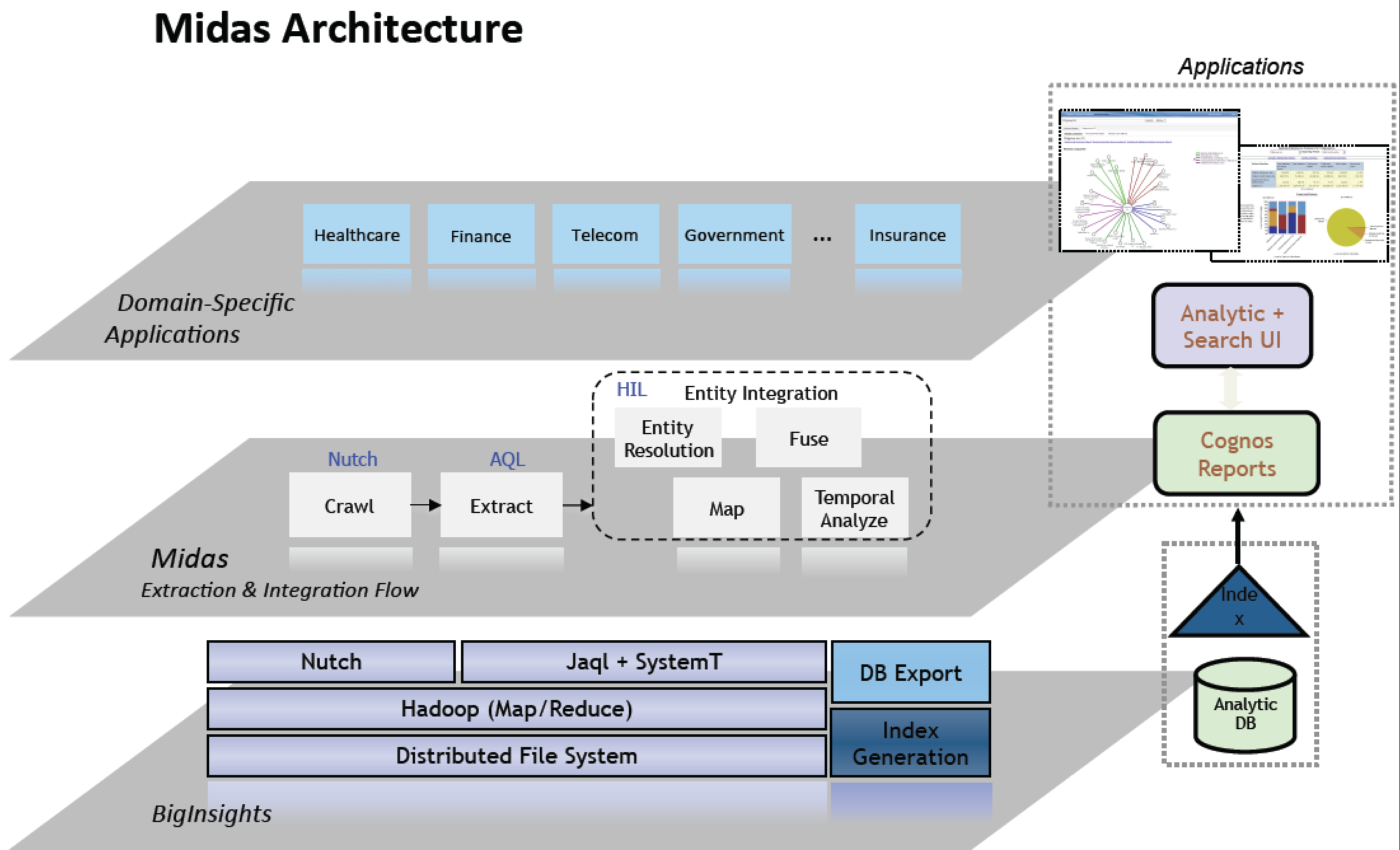
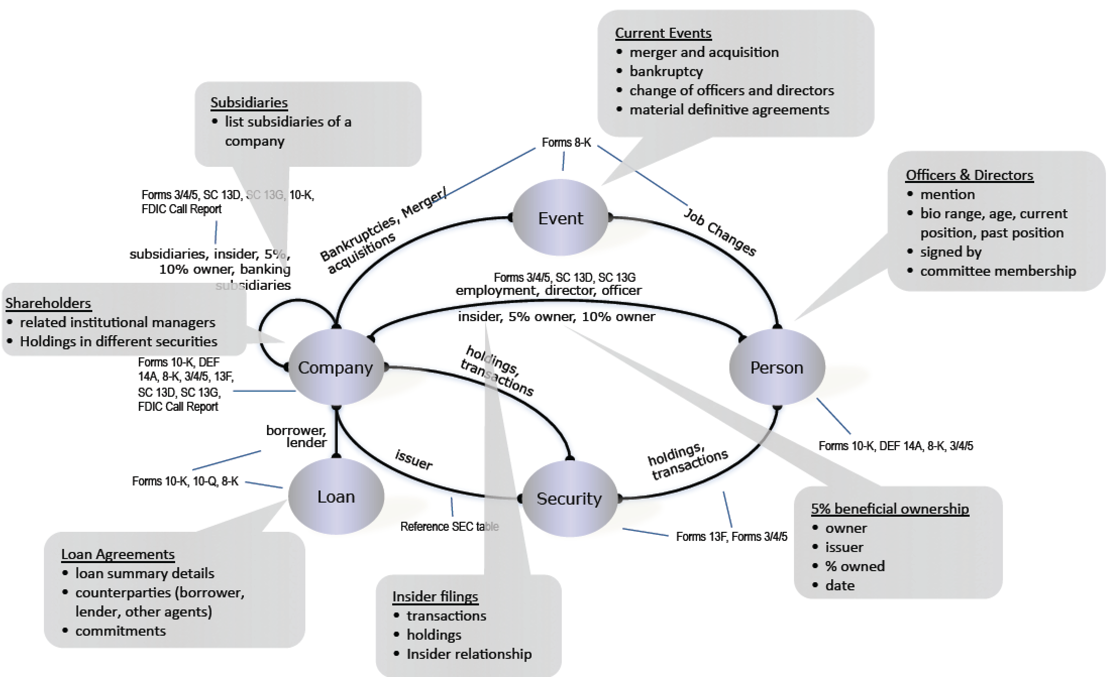
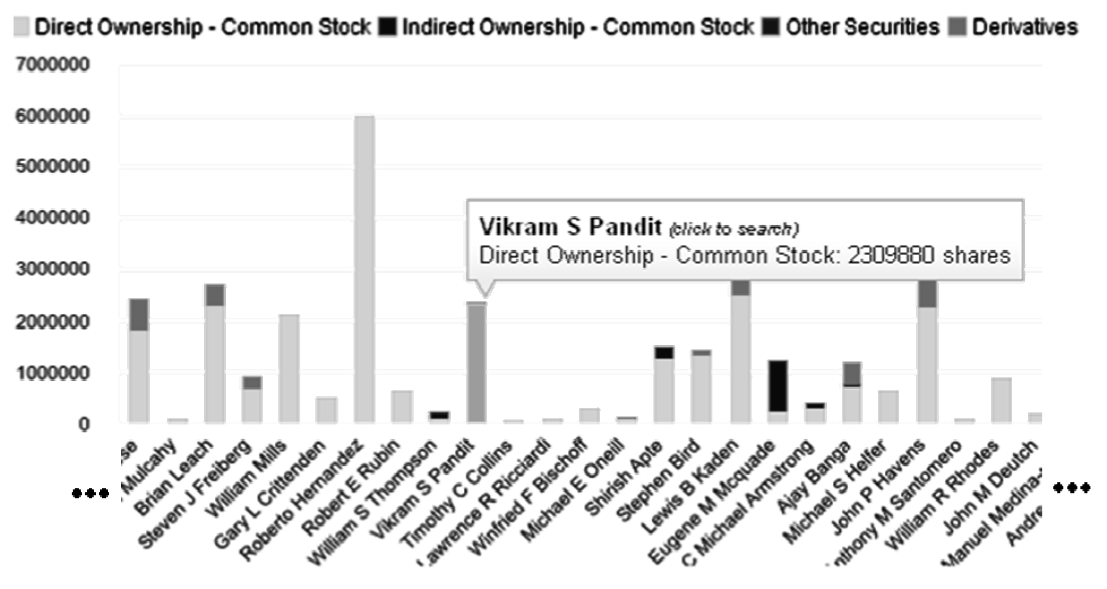
![]()
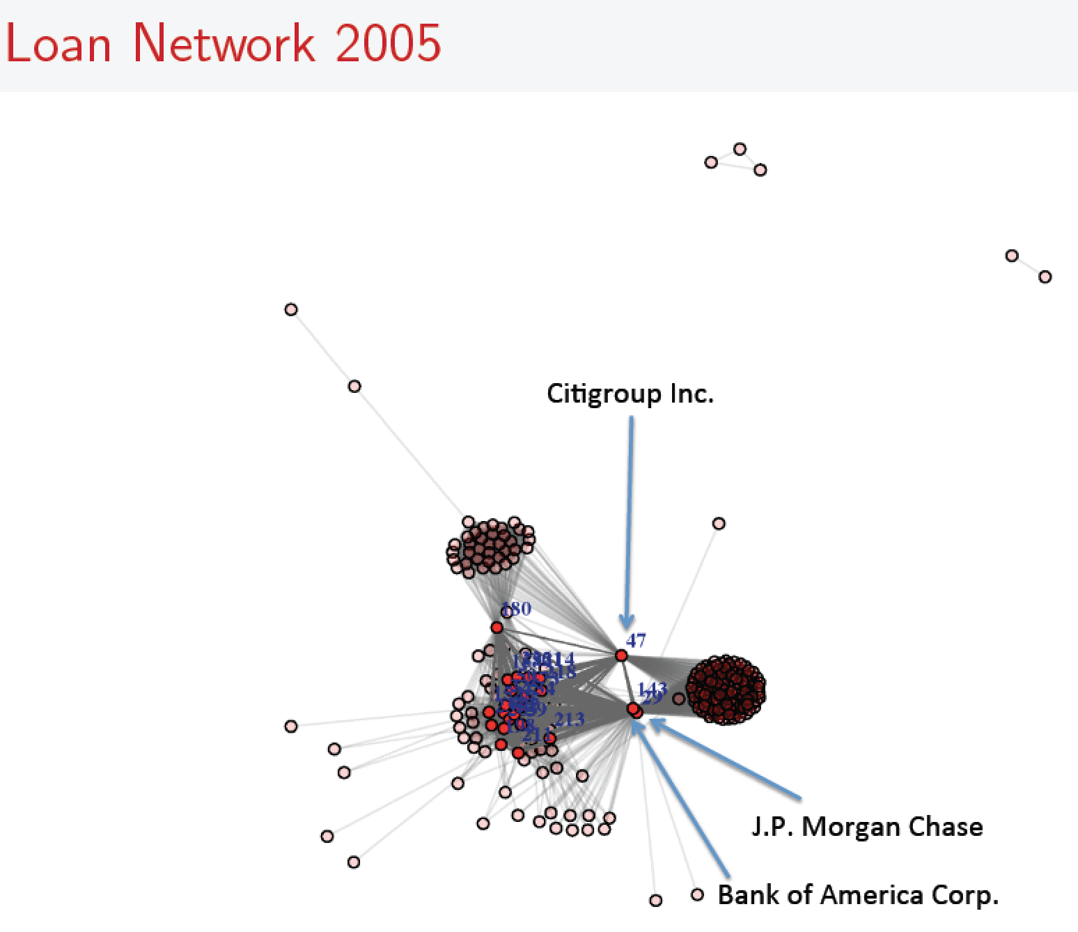
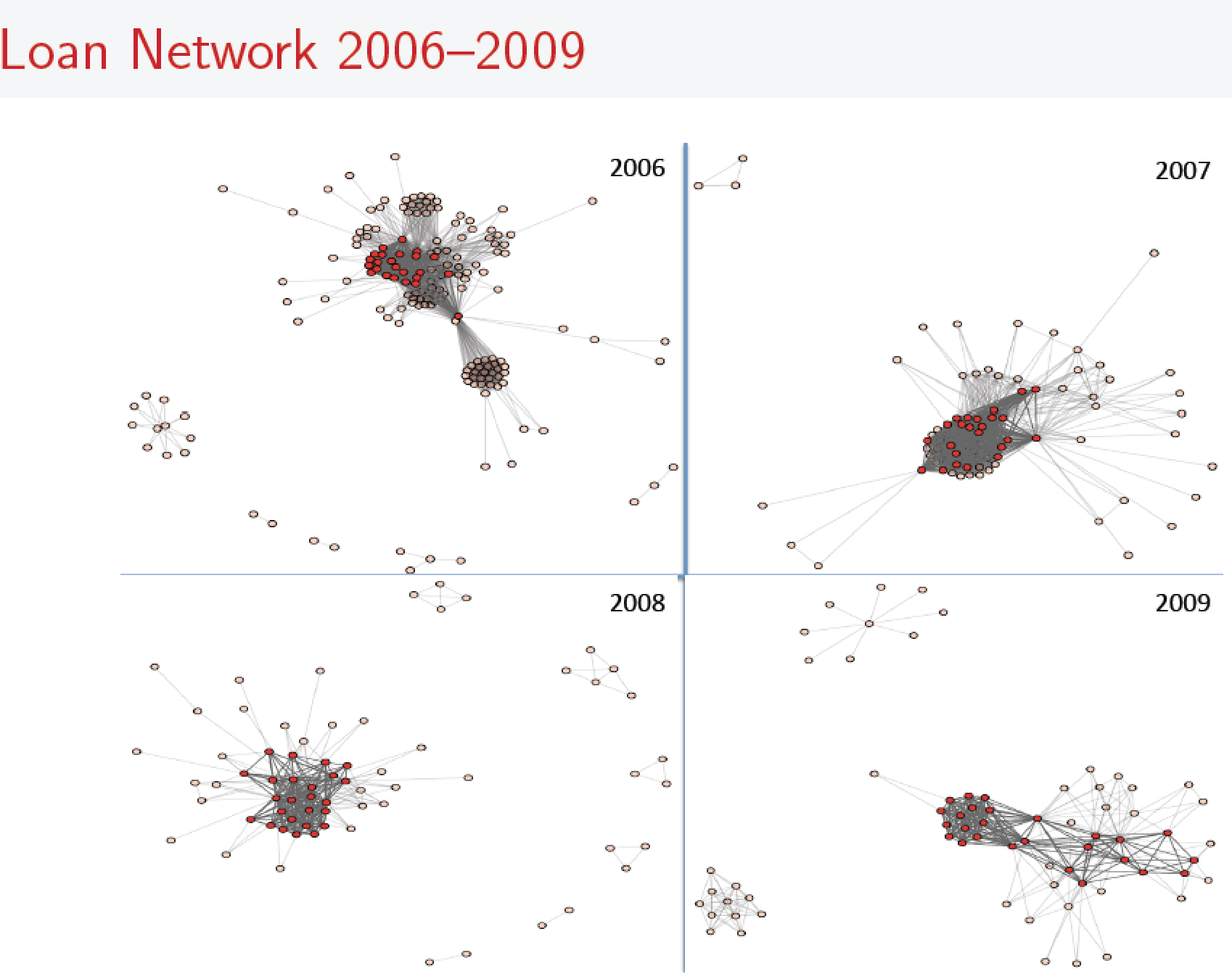
7.47.2 Stock Twits
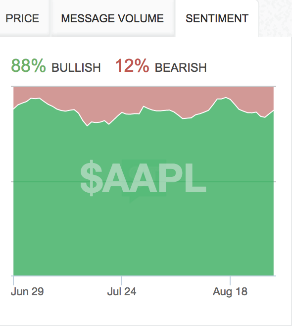
7.47.3 iSentium
7.47.4 RavenPack
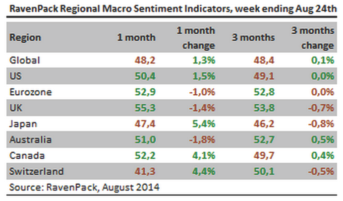
7.47.5 Possibile Applications for Finance Firms
An illustrative list of applications for finance firms is as follows:
- Monitoring corporate buzz.
- Analyzing textual data to detect, analyze, and understand the more profitable customers or products.
- Targeting new clients.
- Customer retention, which is a huge issue. Text mining complaints to prioritize customer remedial action makes a huge difference, especially in the insurance business.
- Lending activity - automated management of profiling information for lending screening.
- Market prediction and trading.
- Risk management.
- Automated financial analysts.
- Financial forensics to prevent rogue employees from inflicting large losses.
- Fraud detection.
- Detecting market manipulation.
- Social network analysis of clients.
- Measuring institutional risk from systemic risk.
7.48 Latent Semantic Analysis (LSA)
Latent Semantic Analysis (LSA) is an approach for reducing the dimension of the Term-Document Matrix (TDM), or the corresponding Document-Term Matrix (DTM), in general used interchangeably, unless a specific one is invoked. Dimension reduction of the TDM offers two benefits:
The DTM is usually a sparse matrix, and sparseness means that our algorithms have to work harder on missing data, which is clearly wasteful. Some of this sparseness is attenuated by applying LSA to the TDM.
The problem of synonymy also exists in the TDM, which usually contains thousands of terms (words). Synonymy arises becauses many words have similar meanings, i.e., redundancy exists in the list of terms. LSA mitigates this redundancy, as we shall see through the ensuing anaysis of LSA.
While not precisely the same thing, think of LSA in the text domain as analogous to PCA in the data domain.
7.48.1 How is LSA implemented using SVD?
LSA is the application of Singular Value Decomposition (SVD) to the TDM, extracted from a text corpus. Define the TDM to be a matrix \(M \in {\cal R}^{m \times n}\), where \(m\) is the number of terms and \(n\) is the number of documents.
The SVD of matrix \(M\) is given by
\[ M = T \cdot S \cdot D^\top \]
where \(T \in {\cal R}^{m \times n}\) and \(D \in {\cal R}^{n \times n}\) are orthonormal to each other, and \(S \in {\cal R}^{n \times n}\) is the “singluar values” matrix, i.e., a diagonal matrix with singular values on the diagonal. These values denote the relative importance of the terms in the TDM.
7.48.2 Example
Create a temporary directory and add some documents to it. This is a modification of the example in the lsa package
system("mkdir D")
write( c("blue", "red", "green"), file=paste("D", "D1.txt", sep="/"))
write( c("black", "blue", "red"), file=paste("D", "D2.txt", sep="/"))
write( c("yellow", "black", "green"), file=paste("D", "D3.txt", sep="/"))
write( c("yellow", "red", "black"), file=paste("D", "D4.txt", sep="/"))Create a TDM using the textmatrix function.
library(lsa)
tdm = textmatrix("D",minWordLength=1)
print(tdm)## docs
## terms D1.txt D2.txt D3.txt D4.txt
## blue 1 1 0 0
## green 1 0 1 0
## red 1 1 0 1
## black 0 1 1 1
## yellow 0 0 1 1Remove the extra directory.
system("rm -rf D")7.49 Singular Value Decomposition (SVD)
SVD tries to connect the correlation matrix of terms (\(M \cdot M^\top\)) with the correlation matrix of documents (\(M^\top \cdot M\)) through the singular matrix.
To see this connection, note that matrix \(T\) contains the eigenvectors of the correlation matrix of terms. Likewise, the matrix \(D\) contains the eigenvectors of the correlation matrix of documents. To see this, let’s compute
et = eigen(tdm %*% t(tdm))$vectors
print(et)## [,1] [,2] [,3] [,4] [,5]
## [1,] -0.3629044 -6.015010e-01 -0.06829369 3.717480e-01 0.6030227
## [2,] -0.3328695 -2.220446e-16 -0.89347008 5.551115e-16 -0.3015113
## [3,] -0.5593741 -3.717480e-01 0.31014767 -6.015010e-01 -0.3015113
## [4,] -0.5593741 3.717480e-01 0.31014767 6.015010e-01 -0.3015113
## [5,] -0.3629044 6.015010e-01 -0.06829369 -3.717480e-01 0.6030227ed = eigen(t(tdm) %*% tdm)$vectors
print(ed)## [,1] [,2] [,3] [,4]
## [1,] -0.4570561 0.601501 -0.5395366 -0.371748
## [2,] -0.5395366 0.371748 0.4570561 0.601501
## [3,] -0.4570561 -0.601501 -0.5395366 0.371748
## [4,] -0.5395366 -0.371748 0.4570561 -0.6015017.49.1 Dimension reduction of the TDM via LSA
If we wish to reduce the dimension of the latent semantic space to \(k < n\) then we use only the first \(k\) eigenvectors. The lsa function does this automatically.
We call LSA and ask it to automatically reduce the dimension of the TDM using a built-in function dimcalc_share.
res = lsa(tdm,dims=dimcalc_share())
print(res)## $tk
## [,1] [,2]
## blue -0.3629044 -6.015010e-01
## green -0.3328695 -5.551115e-17
## red -0.5593741 -3.717480e-01
## black -0.5593741 3.717480e-01
## yellow -0.3629044 6.015010e-01
##
## $dk
## [,1] [,2]
## D1.txt -0.4570561 -0.601501
## D2.txt -0.5395366 -0.371748
## D3.txt -0.4570561 0.601501
## D4.txt -0.5395366 0.371748
##
## $sk
## [1] 2.746158 1.618034
##
## attr(,"class")
## [1] "LSAspace"We can see that the dimension has been reduced from \(n=4\) to \(n=2\). The output is shown for both the term matrix and the document matrix, both of which have only two columns. Think of these as the two “principal semantic components” of the TDM.
Compare the output of the LSA to the eigenvectors above to see that it is exactly that. The singular values in the ouput are connected to SVD as follows.
7.49.2 LSA and SVD: the connection?
First of all we see that the lsa function is nothing but the svd function in base R.
res2 = svd(tdm)
print(res2)## $d
## [1] 2.746158 1.618034 1.207733 0.618034
##
## $u
## [,1] [,2] [,3] [,4]
## [1,] -0.3629044 -6.015010e-01 0.06829369 3.717480e-01
## [2,] -0.3328695 -5.551115e-17 0.89347008 -3.455569e-15
## [3,] -0.5593741 -3.717480e-01 -0.31014767 -6.015010e-01
## [4,] -0.5593741 3.717480e-01 -0.31014767 6.015010e-01
## [5,] -0.3629044 6.015010e-01 0.06829369 -3.717480e-01
##
## $v
## [,1] [,2] [,3] [,4]
## [1,] -0.4570561 -0.601501 0.5395366 -0.371748
## [2,] -0.5395366 -0.371748 -0.4570561 0.601501
## [3,] -0.4570561 0.601501 0.5395366 0.371748
## [4,] -0.5395366 0.371748 -0.4570561 -0.601501The output here is the same as that of LSA except it is provided for \(n=4\). So we have four columns in \(T\) and \(D\) rather than two. Compare the results here to the previous two slides to see the connection.
7.49.3 What is the rank of the TDM?
We may reconstruct the TDM using the result of the LSA.
tdm_lsa = res$tk %*% diag(res$sk) %*% t(res$dk)
print(tdm_lsa)## D1.txt D2.txt D3.txt D4.txt
## blue 1.0409089 0.8995016 -0.1299115 0.1758948
## green 0.4178005 0.4931970 0.4178005 0.4931970
## red 1.0639006 1.0524048 0.3402938 0.6051912
## black 0.3402938 0.6051912 1.0639006 1.0524048
## yellow -0.1299115 0.1758948 1.0409089 0.8995016We see the new TDM after the LSA operation, it has non-integer frequency counts, but it may be treated in the same way as the original TDM. The document vectors populate a slightly different hyperspace.
LSA reduces the rank of the correlation matrix of terms \(M \cdot M^\top\) to \(n=2\). Here we see the rank before and after LSA.
library(Matrix)
print(rankMatrix(tdm))## [1] 4
## attr(,"method")
## [1] "tolNorm2"
## attr(,"useGrad")
## [1] FALSE
## attr(,"tol")
## [1] 1.110223e-15print(rankMatrix(tdm_lsa))## [1] 2
## attr(,"method")
## [1] "tolNorm2"
## attr(,"useGrad")
## [1] FALSE
## attr(,"tol")
## [1] 1.110223e-157.50 Topic Analysis with Latent Dirichlet Allocation (LDA)
7.50.1 What does LDA have to do with LSA?
It is similar to LSA, in that it seeks to find the most related words and cluster them into topics. It uses a Bayesian approach to do this, but more on that later. Here, let’s just do an example to see how we might use the topicmodels package.
#Load the package
library(topicmodels)
#Load data on news articles from Associated Press
data(AssociatedPress)
print(dim(AssociatedPress))## [1] 2246 10473This is a large DTM (not TDM). It has more than 10,000 terms, and more than 2,000 documents. This is very large and LDA will take some time, so let’s run it on a subset of the documents.
dtm = AssociatedPress[1:100,]
dim(dtm)## [1] 100 10473Now we run LDA on this data set.
#Set parameters for Gibbs sampling
burnin = 4000
iter = 2000
thin = 500
seed = list(2003,5,63,100001,765)
nstart = 5
best = TRUE
#Number of topics
k = 5#Run LDA
res <-LDA(dtm, k, method="Gibbs", control = list(nstart = nstart, seed = seed, best = best, burnin = burnin, iter = iter, thin = thin))
#Show topics
res.topics = as.matrix(topics(res))
print(res.topics)## [,1]
## [1,] 5
## [2,] 4
## [3,] 5
## [4,] 1
## [5,] 1
## [6,] 4
## [7,] 2
## [8,] 1
## [9,] 5
## [10,] 5
## [11,] 5
## [12,] 3
## [13,] 1
## [14,] 4
## [15,] 2
## [16,] 3
## [17,] 1
## [18,] 1
## [19,] 2
## [20,] 3
## [21,] 5
## [22,] 2
## [23,] 2
## [24,] 1
## [25,] 2
## [26,] 4
## [27,] 4
## [28,] 2
## [29,] 4
## [30,] 3
## [31,] 2
## [32,] 1
## [33,] 4
## [34,] 1
## [35,] 5
## [36,] 4
## [37,] 1
## [38,] 4
## [39,] 4
## [40,] 2
## [41,] 2
## [42,] 2
## [43,] 1
## [44,] 1
## [45,] 5
## [46,] 3
## [47,] 2
## [48,] 3
## [49,] 1
## [50,] 4
## [51,] 1
## [52,] 2
## [53,] 3
## [54,] 1
## [55,] 3
## [56,] 4
## [57,] 4
## [58,] 2
## [59,] 5
## [60,] 2
## [61,] 2
## [62,] 3
## [63,] 2
## [64,] 1
## [65,] 2
## [66,] 4
## [67,] 5
## [68,] 2
## [69,] 4
## [70,] 5
## [71,] 5
## [72,] 5
## [73,] 2
## [74,] 5
## [75,] 2
## [76,] 1
## [77,] 1
## [78,] 1
## [79,] 3
## [80,] 5
## [81,] 1
## [82,] 3
## [83,] 5
## [84,] 3
## [85,] 3
## [86,] 5
## [87,] 2
## [88,] 5
## [89,] 2
## [90,] 5
## [91,] 3
## [92,] 1
## [93,] 1
## [94,] 4
## [95,] 3
## [96,] 4
## [97,] 4
## [98,] 4
## [99,] 5
## [100,] 5#Show top terms
res.terms = as.matrix(terms(res,10))
print(res.terms)## Topic 1 Topic 2 Topic 3 Topic 4 Topic 5
## [1,] "i" "percent" "new" "soviet" "police"
## [2,] "people" "year" "york" "government" "central"
## [3,] "state" "company" "expected" "official" "man"
## [4,] "years" "last" "states" "two" "monday"
## [5,] "bush" "new" "officials" "union" "friday"
## [6,] "president" "bank" "program" "officials" "city"
## [7,] "get" "oil" "california" "war" "four"
## [8,] "told" "prices" "week" "president" "school"
## [9,] "administration" "report" "air" "world" "high"
## [10,] "dukakis" "million" "help" "leaders" "national"#Show topic probabilities
res.topicProbs = as.data.frame(res@gamma)
print(res.topicProbs)## V1 V2 V3 V4 V5
## 1 0.19169329 0.06070288 0.04472843 0.10223642 0.60063898
## 2 0.12149533 0.14330218 0.08099688 0.58255452 0.07165109
## 3 0.27213115 0.04262295 0.05901639 0.07868852 0.54754098
## 4 0.29571984 0.16731518 0.19844358 0.19455253 0.14396887
## 5 0.31896552 0.15517241 0.20689655 0.14655172 0.17241379
## 6 0.30360934 0.08492569 0.08492569 0.46284501 0.06369427
## 7 0.17050691 0.40092166 0.15668203 0.17050691 0.10138249
## 8 0.37142857 0.15238095 0.14285714 0.20000000 0.13333333
## 9 0.19298246 0.17543860 0.19298246 0.19298246 0.24561404
## 10 0.19879518 0.16265060 0.17469880 0.18674699 0.27710843
## 11 0.21212121 0.20202020 0.16161616 0.15151515 0.27272727
## 12 0.20143885 0.15827338 0.25899281 0.17985612 0.20143885
## 13 0.41395349 0.16279070 0.18139535 0.12558140 0.11627907
## 14 0.17948718 0.17948718 0.12820513 0.30769231 0.20512821
## 15 0.05135952 0.78247734 0.06344411 0.06042296 0.04229607
## 16 0.09770115 0.24712644 0.35632184 0.14942529 0.14942529
## 17 0.43103448 0.18103448 0.09051724 0.10775862 0.18965517
## 18 0.67857143 0.04591837 0.06377551 0.08418367 0.12755102
## 19 0.07083333 0.70000000 0.08750000 0.07500000 0.06666667
## 20 0.15196078 0.05637255 0.69117647 0.04656863 0.05392157
## 21 0.21782178 0.11881188 0.12871287 0.15841584 0.37623762
## 22 0.16666667 0.30000000 0.16666667 0.16666667 0.20000000
## 23 0.19298246 0.21052632 0.17543860 0.21052632 0.21052632
## 24 0.31775701 0.20560748 0.16822430 0.18691589 0.12149533
## 25 0.05121951 0.65121951 0.15365854 0.08536585 0.05853659
## 26 0.11740891 0.09311741 0.08502024 0.37246964 0.33198381
## 27 0.06583072 0.05956113 0.10658307 0.68338558 0.08463950
## 28 0.15068493 0.30136986 0.12328767 0.26027397 0.16438356
## 29 0.07860262 0.04148472 0.05676856 0.68995633 0.13318777
## 30 0.13968254 0.17142857 0.46031746 0.07936508 0.14920635
## 31 0.08405172 0.74784483 0.07112069 0.05172414 0.04525862
## 32 0.66137566 0.10846561 0.06349206 0.07407407 0.09259259
## 33 0.14655172 0.18103448 0.15517241 0.41379310 0.10344828
## 34 0.29605263 0.19736842 0.21052632 0.13157895 0.16447368
## 35 0.08080808 0.05050505 0.10437710 0.07070707 0.69360269
## 36 0.13333333 0.07878788 0.08484848 0.46666667 0.23636364
## 37 0.46202532 0.08227848 0.12974684 0.16139241 0.16455696
## 38 0.09442060 0.07296137 0.12017167 0.64377682 0.06866953
## 39 0.11764706 0.08359133 0.10526316 0.62538700 0.06811146
## 40 0.10869565 0.56521739 0.14492754 0.07246377 0.10869565
## 41 0.07671958 0.43650794 0.16137566 0.25396825 0.07142857
## 42 0.11445783 0.57831325 0.11445783 0.09036145 0.10240964
## 43 0.55793991 0.10944206 0.08798283 0.09442060 0.15021459
## 44 0.40939597 0.10067114 0.22818792 0.12751678 0.13422819
## 45 0.20000000 0.15121951 0.12682927 0.25853659 0.26341463
## 46 0.14828897 0.11406844 0.56653992 0.08365019 0.08745247
## 47 0.09929078 0.41134752 0.13475177 0.22695035 0.12765957
## 48 0.20129870 0.07467532 0.54870130 0.10714286 0.06818182
## 49 0.46800000 0.09600000 0.18400000 0.10400000 0.14800000
## 50 0.22955145 0.08179420 0.05013193 0.60158311 0.03693931
## 51 0.28368794 0.17730496 0.18439716 0.14893617 0.20567376
## 52 0.12977099 0.45801527 0.12977099 0.18320611 0.09923664
## 53 0.10507246 0.14492754 0.55072464 0.06884058 0.13043478
## 54 0.42647059 0.13725490 0.15196078 0.15686275 0.12745098
## 55 0.11881188 0.19801980 0.44554455 0.08910891 0.14851485
## 56 0.22857143 0.15714286 0.13571429 0.37142857 0.10714286
## 57 0.15294118 0.07058824 0.06117647 0.66823529 0.04705882
## 58 0.11494253 0.49425287 0.14367816 0.12068966 0.12643678
## 59 0.13278008 0.04979253 0.13692946 0.26556017 0.41493776
## 60 0.16666667 0.31666667 0.16666667 0.16666667 0.18333333
## 61 0.06796117 0.73786408 0.08090615 0.04854369 0.06472492
## 62 0.12680115 0.12968300 0.58213256 0.12103746 0.04034582
## 63 0.07902736 0.72948328 0.09118541 0.05471125 0.04559271
## 64 0.44285714 0.12142857 0.14285714 0.13214286 0.16071429
## 65 0.19540230 0.31034483 0.19540230 0.14942529 0.14942529
## 66 0.18518519 0.22222222 0.17037037 0.28888889 0.13333333
## 67 0.07024793 0.07851240 0.08677686 0.04545455 0.71900826
## 68 0.10181818 0.48000000 0.14909091 0.12727273 0.14181818
## 69 0.12307692 0.15384615 0.10000000 0.43076923 0.19230769
## 70 0.12745098 0.07352941 0.14215686 0.13235294 0.52450980
## 71 0.21582734 0.10791367 0.16546763 0.14388489 0.36690647
## 72 0.17560976 0.11219512 0.17073171 0.15609756 0.38536585
## 73 0.12280702 0.46198830 0.07602339 0.23976608 0.09941520
## 74 0.20535714 0.16964286 0.17857143 0.14285714 0.30357143
## 75 0.07567568 0.47027027 0.11891892 0.19459459 0.14054054
## 76 0.67310789 0.15619968 0.07407407 0.05152979 0.04508857
## 77 0.63834423 0.07189542 0.09150327 0.11546841 0.08278867
## 78 0.61504425 0.09292035 0.11946903 0.11504425 0.05752212
## 79 0.10971787 0.07523511 0.65830721 0.07210031 0.08463950
## 80 0.11111111 0.08666667 0.11111111 0.05777778 0.63333333
## 81 0.49681529 0.03821656 0.15286624 0.14437367 0.16772824
## 82 0.20111732 0.17318436 0.24022346 0.15642458 0.22905028
## 83 0.10731707 0.15609756 0.11219512 0.23902439 0.38536585
## 84 0.26016260 0.10569106 0.36585366 0.13008130 0.13821138
## 85 0.11525424 0.10508475 0.39322034 0.30508475 0.08135593
## 86 0.15454545 0.06060606 0.15757576 0.09696970 0.53030303
## 87 0.08301887 0.67924528 0.07924528 0.09433962 0.06415094
## 88 0.16666667 0.15972222 0.22916667 0.11805556 0.32638889
## 89 0.12389381 0.47787611 0.09734513 0.14159292 0.15929204
## 90 0.12389381 0.11061947 0.23008850 0.10176991 0.43362832
## 91 0.19724771 0.11009174 0.30275229 0.16972477 0.22018349
## 92 0.33854167 0.13541667 0.12500000 0.11458333 0.28645833
## 93 0.40131579 0.13815789 0.10526316 0.18421053 0.17105263
## 94 0.06930693 0.10231023 0.09240924 0.67656766 0.05940594
## 95 0.09130435 0.15000000 0.65434783 0.03043478 0.07391304
## 96 0.13370474 0.13091922 0.12256267 0.49303621 0.11977716
## 97 0.06709265 0.06070288 0.11501597 0.60383387 0.15335463
## 98 0.16438356 0.16438356 0.17808219 0.28767123 0.20547945
## 99 0.06274510 0.08235294 0.16470588 0.06666667 0.62352941
## 100 0.11627907 0.20465116 0.11162791 0.16744186 0.40000000#Check that each term is allocated to all topics
print(rowSums(res.topicProbs))## [1] 1 1 1 1 1 1 1 1 1 1 1 1 1 1 1 1 1 1 1 1 1 1 1 1 1 1 1 1 1 1 1 1 1 1 1
## [36] 1 1 1 1 1 1 1 1 1 1 1 1 1 1 1 1 1 1 1 1 1 1 1 1 1 1 1 1 1 1 1 1 1 1 1
## [71] 1 1 1 1 1 1 1 1 1 1 1 1 1 1 1 1 1 1 1 1 1 1 1 1 1 1 1 1 1 1Note that the highest probability in each row assigns each document to a topic.
7.51 LDA Explained (Briefly)
Latent Dirichlet Allocation (LDA) was created by David Blei, Andrew Ng, and Michael Jordan in 2003, see their paper titled “Latent Dirichlet Allocation” in the Journal of Machine Learning Research, pp 993–1022.
The simplest way to think about LDA is as a probability model that connects documents with words and topics. The components are:
- A Vocabulary of \(V\) words, i.e., \(w_1,w_2,...,w_i,...,w_V\), each word indexed by \(i\).
- A Document is a vector of \(N\) words, i.e., \({\bf w}\).
- A Corpus \(D\) is a collection of \(M\) documents, each document indexed by \(j\), i.e. \(d_j\).
Next, we connect the above objects to \(K\) topics, indexed by \(l\), i.e., \(t_l\). We will see that LDA is encapsulated in two matrices: Matrix \(A\) and Matrix \(B\).
7.51.1 Matrix \(A\): Connecting Documents with Topics
- This matrix has documents on the rows, so there are \(M\) rows.
- The topics are on the columns, so there are \(K\) columns.
- Therefore \(A \in {\cal R}^{M \times K}\).
- The row sums equal \(1\), i.e., for each document, we have a probability that it pertains to a given topic, i.e., \(A_{jl} = Pr[t_l | d_j]\), and \(\sum_{l=1}^K A_{jl} = 1\).
7.51.2 Matrix \(B\): Connecting Words with Topics
- This matrix has topics on the rows, so there are \(K\) rows.
- The words are on the columns, so there are \(V\) columns.
- Therefore \(B \in {\cal R}^{K \times V}\).
- The row sums equal \(1\), i.e., for each topic, we have a probability that it pertains to a given word, i.e., \(B_{li} = Pr[w_i | t_l]\), and \(\sum_{i=1}^V B_{li} = 1\).
7.51.3 Distribution of Topics in a Document
- Using Matrix \(A\), we can sample a \(K\)-vector of probabilities of topics for a single document. Denote the probability of this vector as \(p(\theta | \alpha)\), where \(\theta, \alpha \in {\cal R}^K\), \(\theta, \alpha \geq 0\), and \(\sum_l \theta_l = 1\).
- The probability \(p(\theta | \alpha)\) is governed by a Dirichlet distribution, with density function
\[ p(\theta | \alpha) = \frac{\Gamma(\sum_{l=1}^K \alpha_l)}{\prod_{l=1}^K \Gamma(\alpha_l)} \; \prod_{l=1}^K \theta_l^{\alpha_l - 1} \]
where \(\Gamma(\cdot)\) is the Gamma function. - LDA thus gets its name from the use of the Dirichlet distribution, embodied in Matrix \(A\). Since the topics are latent, it explains the rest of the nomenclature. - Given \(\theta\), we sample topics from matrix \(A\) with probability \(p(t | \theta)\).
7.51.4 Distribution of Words and Topics for a Document
- The number of words in a document is assumed to be distributed Poisson with parameter \(\xi\).
- Matrix \(B\) gives the probability of a word appearing in a topic, \(p(w | t)\).
- The topics mixture is given by \(\theta\).
- The joint distribution over \(K\) topics and \(K\) words for a topic mixture is given by
\[ p(\theta, {\bf t}, {\bf w}) = p(\theta | \alpha) \prod_{l=1}^K p(t_l | \theta) p(w_l | t_l) \]
- The marginal distribution for a document’s words comes from integrating out the topic mixture \(\theta\), and summing out the topics \({\bf t}\), i.e.,
\[ p({\bf w}) = \int p(\theta | \alpha) \left(\prod_{l=1}^K \sum_{t_l} p(t_l | \theta) p(w_l | t_l)\; \right) d\theta \]
7.51.5 Likelihood of the entire Corpus
- This is given by:
\[ p(D) = \prod_{j=1}^M \int p(\theta_j | \alpha) \left(\prod_{l=1}^K \sum_{t_{jl}} p(t_l | \theta_j) p(w_l | t_l)\; \right) d\theta_j \]
The goal is to maximize this likelihood by picking the vector \(\alpha\) and the probabilities in the matrix \(B\). (Note that were a Dirichlet distribution not used, then we could directly pick values in Matrices \(A\) and \(B\).)
The computation is undertaken using MCMC with Gibbs sampling as shown in the example earlier.
7.51.6 Examples in Finance
7.51.7 word2vec (explained)
For more details, see: https://www.quora.com/How-does-word2vec-work
A geometrical interpretation: word2vec is a shallow word embedding model. This means that the model learns to map each discrete word id (0 through the number of words in the vocabulary) into a low-dimensional continuous vector-space from their distributional properties observed in some raw text corpus. Geometrically, one may interpret these vectors as tracing out points on the outside surface of a manifold in the “embedded space”. If we initialize these vectors from a spherical gaussian distribution, then you can imagine this manifold to look something like a hypersphere initially.
Let us focus on the CBOW for now. CBOW is trained to predict the target word t from the contextual words that surround it, c, i.e. the goal is to maximize P(t | c) over the training set. I am simplifying somewhat, but you can show that this probability is roughly inversely proportional to the distance between the current vectors assigned to t and to c. Since this model is trained in an online setting (one example at a time), at time T the goal is therefore to take a small step (mediated by the “learning rate”) in order to minimize the distance between the current vectors for t and c (and thereby increase the probability P(t |c)). By repeating this process over the entire training set, we have that vectors for words that habitually co-occur tend to be nudged closer together, and by gradually lowering the learning rate, this process converges towards some final state of the vectors.
By the Distributional Hypothesis (Firth, 1957; see also the Wikipedia page on Distributional semantics), words with similar distributional properties (i.e. that co-occur regularly) tend to share some aspect of semantic meaning. For example, we may find several sentences in the training set such as “citizens of X protested today” where X (the target word t) may be names of cities or countries that are semantically related.
You can therefore interpret each training step as deforming or morphing the initial manifold by nudging the vectors for some words somewhat closer together, and the result, after projecting down to two dimensions, is the familiar t-SNE visualizations where related words cluster together (e.g. Word representations for NLP).
For the skipgram, the direction of the prediction is simply inverted, i.e. now we try to predict P(citizens | X), P(of | X), etc. This turns out to learn finer-grained vectors when one trains over more data. The main reason is that the CBOW smooths over a lot of the distributional statistics by averaging over all context words while the skipgram does not. With little data, this “regularizing” effect of the CBOW turns out to be helpful, but since data is the ultimate regularizer the skipgram is able to extract more information when more data is available.
There’s a bit more going on behind the scenes, but hopefully this helps to give a useful geometrical intuition as to how these models work.