Chapter 11 Truncate and Estimate: Limited Dependent Variables
11.1 Maximum-Likelihood Estimation (MLE)
Suppose we wish to fit data to a given distribution, then we may use this technique to do so. Many of the data fitting procedures need to use MLE. MLE is a general technique, and applies widely. It is also a fundamental approach to many estimation tools in econometrics. Here we recap this.
Let’s say we have a series of data \(x\), with \(T\) observations. If \(x \sim N(\mu,\sigma^2)\), then \[\begin{equation} \mbox{density function:} \quad f(x) = \frac{1}{\sqrt{2\pi\sigma^2}} \exp\left[-\frac{1}{2}\frac{(x-\mu)^2}{\sigma^2} \right] \end{equation}\] \[\begin{equation} N(x) = 1 - N(-x) \end{equation}\] \[\begin{equation} F(x) = \int_{-\infty}^x f(u) du \end{equation}\]The standard normal distribution is \(x \sim N(0,1)\). For the standard normal distribution: \(F(0) = \frac{1}{2}\).
The likelihood of the entire series is
\[\begin{equation} \prod_{t=1}^T f[R(t)] \end{equation}\] It is easier (computationally) to maximize \[\begin{equation} \max_{\mu,\sigma} \; {\cal L} \equiv \sum_{t=1}^T \ln f[R(t)] \end{equation}\]known as the log-likelihood.
11.2 Implementation
This is easily done in R. First we create the log-likelihood function, so you can see how functions are defined in R. Second, we optimize the log-likelihood, i.e., we find the maximum value, hence it is known as maximum log-likelihood estimation (MLE).
#LOG-LIKELIHOOD FUNCTION
LL = function(params,x) {
    mu = params[1]; sigsq = params[2]
    f = (1/sqrt(2*pi*sigsq))*exp(-0.5*(x-mu)^2/sigsq)
    LL = -sum(log(f))
}
#GENERATE DATA FROM A NORMAL DISTRIBUTION
x = rnorm(10000, mean=5, sd=3)
#MAXIMIZE LOG-LIKELIHOOD
params = c(4,2) #Create starting guess for parameters
res = nlm(LL,params,x)
print(res)## $minimum
## [1] 25257.34
##
## $estimate
## [1] 4.965689 9.148508
##
## $gradient
## [1] 0.0014777011 -0.0002584778
##
## $code
## [1] 1
##
## $iterations
## [1] 11We can see that the result was a fitted normal distribution with mean close to 5, and variance close to 9, the square root of which is roughly the same as the distribution from which the data was originally generated. Further, notice that the gradient is zero for both parameters, as it should be when the maximum is reached.
11.3 Logit and Probit Models
Usually we run regressions using continuous variables for the dependent (\(y\)) variables, such as, for example, when we regress income on education. Sometimes however, the dependent variable may be discrete, and could be binomial or multinomial. That is, the dependent variable is limited. In such cases, we need a different approach.
Discrete dependent variables are a special case of limited dependent variables. The Logit and Probit models we look at here are examples of discrete dependent variable models. Such models are also often called qualitative response (QR) models.
In particular, when the variable is binary, i.e., takes values of \(\{0,1\}\), then we get a probability model. If we just regressed the left hand side variables of ones and zeros on a suite of right hand side variables we could of course fit a linear regression. Then if we took another observation with values for the right hand side, i.e., \(x = \{x_1,x_2,\ldots,x_k\}\), we could compute the value of the \(y\) variable using the fitted coefficients. But of course, this value will not be exactly 0 or 1, except by unlikely coincidence. Nor will this value lie in the range \((0,1)\).
There is also a relationship to classifier models. In classifier models, we are interested in allocating observations to categories. In limited dependent models we also want to explain the reasons (i.e., find explanatory variables) for the allocation across categories.
Some examples of such models are to explain whether a person is employed or not, whether a firm is syndicated or not, whether a firm is solvent or not, which field of work is chosen by graduates, where consumers shop, whether they choose Coke versus Pepsi, etc.
These fitted values might not even lie between 0 and 1 with a linear regression. However, if we used a carefully chosen nonlinear regression function, then we could ensure that the fitted values of \(y\) are restricted to the range \((0,1)\), and then we would get a model where we fitted a probability. There are two such model forms that are widely used: (a) Logit, also known as a logistic regression, and (b) Probit models. We look at each one in turn.
11.4 Logit
A logit model takes the following form:
\[\begin{equation} y = \frac{e^{f(x)}}{1+e^{f(x)}}, \quad f(x) = \beta_0 + \beta_1 x_1 + \ldots \beta_k x_k \end{equation}\]We are interested in fitting the coefficients \(\{\beta_0,\beta_1, \ldots, \beta_k\}\). Note that, irrespective of the coefficients, \(f(x) \in (-\infty,+\infty)\), but \(y \in (0,1)\). When \(f(x) \rightarrow -\infty\), \(y \rightarrow 0\), and when \(f(x) \rightarrow +\infty\), \(y \rightarrow 1\). We also write this model as
\[\begin{equation} y = \frac{e^{\beta' x}}{1+e^{\beta' x}} \equiv \Lambda(\beta' x) \end{equation}\]where \(\Lambda\) (lambda) is for logit.
The model generates a \(S\)-shaped curve for \(y\), and we can plot it as follows. The fitted value of \(y\) is nothing but the probability that \(y=1\).
logit = function(fx) { res = exp(fx)/(1+exp(fx)) }
fx = seq(-4,4,0.01)
y = logit(fx)
plot(fx,y,type="l",xlab="x",ylab="f(x)",col="blue",lwd=3)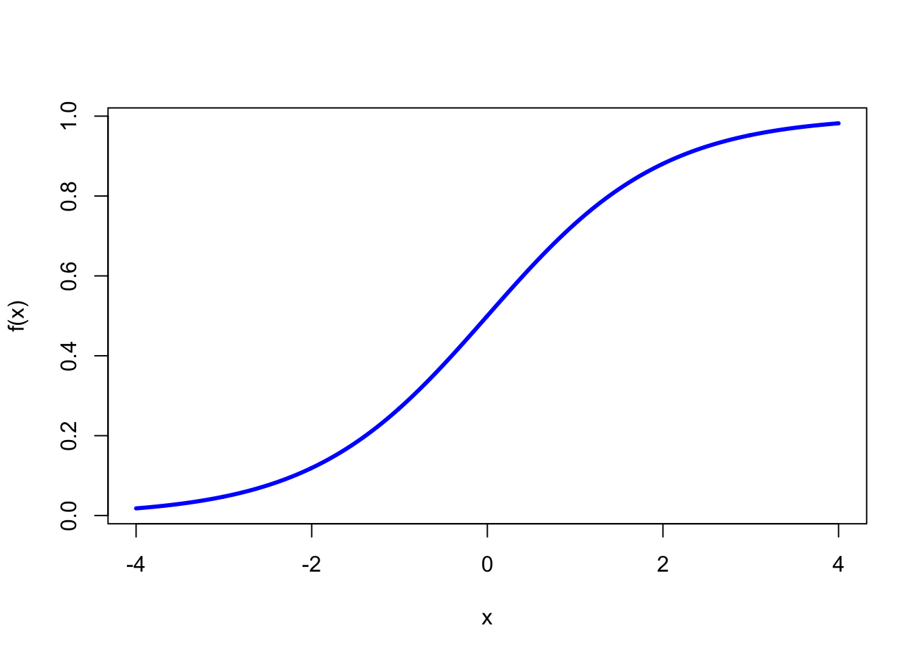
11.4.1 Example
For the NCAA data, take the top 32 teams and make their dependent variable 1, and that of the bottom 32 teams zero. Therefore, the teams that have \(y=1\) are those that did not lose in the first round of the playoffs, and the teams that have \(y=0\) are those that did. Estimation is done by maximizing the log-likelihood.
ncaa = read.table("DSTMAA_data/ncaa.txt",header=TRUE)

y1 = 1:32
y1 = y1*0+1
y2 = y1*0
y = c(y1,y2)
print(y)
## [1] 1 1 1 1 1 1 1 1 1 1 1 1 1 1 1 1 1 1 1 1 1 1 1 1 1 1 1 1 1 1 1 1 0 0 0
## [36] 0 0 0 0 0 0 0 0 0 0 0 0 0 0 0 0 0 0 0 0 0 0 0 0 0 0 0 0 0x = as.matrix(ncaa[4:14])
h = glm(y~x, family=binomial(link="logit"))
names(h)## [1] "coefficients" "residuals" "fitted.values"
## [4] "effects" "R" "rank"
## [7] "qr" "family" "linear.predictors"
## [10] "deviance" "aic" "null.deviance"
## [13] "iter" "weights" "prior.weights"
## [16] "df.residual" "df.null" "y"
## [19] "converged" "boundary" "model"
## [22] "call" "formula" "terms"
## [25] "data" "offset" "control"
## [28] "method" "contrasts" "xlevels"print(logLik(h))## 'log Lik.' -21.44779 (df=12)summary(h)##
## Call:
## glm(formula = y ~ x, family = binomial(link = "logit"))
##
## Deviance Residuals:
## Min 1Q Median 3Q Max
## -1.80174 -0.40502 -0.00238 0.37584 2.31767
##
## Coefficients:
## Estimate Std. Error z value Pr(>|z|)
## (Intercept) -45.83315 14.97564 -3.061 0.00221 **
## xPTS -0.06127 0.09549 -0.642 0.52108
## xREB 0.49037 0.18089 2.711 0.00671 **
## xAST 0.16422 0.26804 0.613 0.54010
## xTO -0.38405 0.23434 -1.639 0.10124
## xA.T 1.56351 3.17091 0.493 0.62196
## xSTL 0.78360 0.32605 2.403 0.01625 *
## xBLK 0.07867 0.23482 0.335 0.73761
## xPF 0.02602 0.13644 0.191 0.84874
## xFG 46.21374 17.33685 2.666 0.00768 **
## xFT 10.72992 4.47729 2.397 0.01655 *
## xX3P 5.41985 5.77966 0.938 0.34838
## ---
## Signif. codes: 0 '***' 0.001 '**' 0.01 '*' 0.05 '.' 0.1 ' ' 1
##
## (Dispersion parameter for binomial family taken to be 1)
##
## Null deviance: 88.723 on 63 degrees of freedom
## Residual deviance: 42.896 on 52 degrees of freedom
## AIC: 66.896
##
## Number of Fisher Scoring iterations: 6h$fitted.values## 1 2 3 4 5
## 0.9998267965 0.9983229192 0.9686755530 0.9909359265 0.9977011039
## 6 7 8 9 10
## 0.9639506326 0.5381841865 0.9505255187 0.4329829232 0.7413280575
## 11 12 13 14 15
## 0.9793554057 0.7273235463 0.2309261473 0.9905414749 0.7344407215
## 16 17 18 19 20
## 0.9936312074 0.2269619354 0.8779507370 0.2572796426 0.9335376447
## 21 22 23 24 25
## 0.9765843274 0.7836742557 0.9967552281 0.9966486903 0.9715110760
## 26 27 28 29 30
## 0.0681674628 0.4984153630 0.9607522159 0.8624544140 0.6988578200
## 31 32 33 34 35
## 0.9265057217 0.7472357037 0.5589318497 0.2552381741 0.0051790298
## 36 37 38 39 40
## 0.4394307950 0.0205919396 0.0545333361 0.0100662111 0.0995262051
## 41 42 43 44 45
## 0.1219394290 0.0025416737 0.3191888357 0.0149772804 0.0685930622
## 46 47 48 49 50
## 0.3457439539 0.0034943441 0.5767386617 0.5489544863 0.4637012227
## 51 52 53 54 55
## 0.2354894587 0.0487342700 0.6359622098 0.8027221707 0.0003240393
## 56 57 58 59 60
## 0.0479116454 0.3422867567 0.4649889328 0.0547385409 0.0722894447
## 61 62 63 64
## 0.0228629774 0.0002730981 0.0570387301 0.283062876011.5 Probit
Probit has essentially the same idea as the logit except that the probability function is replaced by the normal distribution. The nonlinear regression equation is as follows:
\[\begin{equation} y = \Phi[f(x)], \quad f(x) = \beta_0 + \beta_1 x_1 + \ldots \beta_k x_k \end{equation}\]where \(\Phi(.)\) is the cumulative normal probability function. Again, irrespective of the coefficients, \(f(x) \in (-\infty,+\infty)\), but \(y \in (0,1)\). When \(f(x) \rightarrow -\infty\), \(y \rightarrow 0\), and when \(f(x) \rightarrow +\infty\), \(y \rightarrow 1\).
We can redo the same previous logit model using a probit instead:
h = glm(y~x, family=binomial(link="probit"))
print(logLik(h))
## 'log Lik.' -21.27924 (df=12)summary(h)##
## Call:
## glm(formula = y ~ x, family = binomial(link = "probit"))
##
## Deviance Residuals:
## Min 1Q Median 3Q Max
## -1.76353 -0.41212 -0.00031 0.34996 2.24568
##
## Coefficients:
## Estimate Std. Error z value Pr(>|z|)
## (Intercept) -26.28219 8.09608 -3.246 0.00117 **
## xPTS -0.03463 0.05385 -0.643 0.52020
## xREB 0.28493 0.09939 2.867 0.00415 **
## xAST 0.10894 0.15735 0.692 0.48874
## xTO -0.23742 0.13642 -1.740 0.08180 .
## xA.T 0.71485 1.86701 0.383 0.70181
## xSTL 0.45963 0.18414 2.496 0.01256 *
## xBLK 0.03029 0.13631 0.222 0.82415
## xPF 0.01041 0.07907 0.132 0.89529
## xFG 26.58461 9.38711 2.832 0.00463 **
## xFT 6.28278 2.51452 2.499 0.01247 *
## xX3P 3.15824 3.37841 0.935 0.34988
## ---
## Signif. codes: 0 '***' 0.001 '**' 0.01 '*' 0.05 '.' 0.1 ' ' 1
##
## (Dispersion parameter for binomial family taken to be 1)
##
## Null deviance: 88.723 on 63 degrees of freedom
## Residual deviance: 42.558 on 52 degrees of freedom
## AIC: 66.558
##
## Number of Fisher Scoring iterations: 8h$fitted.values## 1 2 3 4 5
## 9.999998e-01 9.999048e-01 9.769711e-01 9.972812e-01 9.997756e-01
## 6 7 8 9 10
## 9.721166e-01 5.590209e-01 9.584564e-01 4.367808e-01 7.362946e-01
## 11 12 13 14 15
## 9.898112e-01 7.262200e-01 2.444006e-01 9.968605e-01 7.292286e-01
## 16 17 18 19 20
## 9.985910e-01 2.528807e-01 8.751178e-01 2.544738e-01 9.435318e-01
## 21 22 23 24 25
## 9.850437e-01 7.841357e-01 9.995601e-01 9.996077e-01 9.825306e-01
## 26 27 28 29 30
## 8.033540e-02 5.101626e-01 9.666841e-01 8.564489e-01 6.657773e-01
## 31 32 33 34 35
## 9.314164e-01 7.481401e-01 5.810465e-01 2.488875e-01 1.279599e-03
## 36 37 38 39 40
## 4.391782e-01 1.020269e-02 5.461190e-02 4.267754e-03 1.067584e-01
## 41 42 43 44 45
## 1.234915e-01 2.665101e-04 3.212605e-01 6.434112e-03 7.362892e-02
## 46 47 48 49 50
## 3.673105e-01 4.875193e-04 6.020993e-01 5.605770e-01 4.786576e-01
## 51 52 53 54 55
## 2.731573e-01 4.485079e-02 6.194202e-01 7.888145e-01 1.630556e-06
## 56 57 58 59 60
## 4.325189e-02 3.899566e-01 4.809365e-01 5.043005e-02 7.330590e-02
## 61 62 63 64
## 1.498018e-02 8.425836e-07 5.515960e-02 3.218696e-0111.6 Analysis
Both these models are just settings in which we are computing binomial (binary) probabilities, i.e.
\[\begin{equation} \mbox{Pr}[y=1] = F(\beta' x) \end{equation}\]where \(\beta\) is a vector of coefficients, and \(x\) is a vector of explanatory variables. \(F\) is the logit/probit function.
\[\begin{equation} {\hat y} = F(\beta' x) \end{equation}\]where \({\hat y}\) is the fitted value of \(y\) for a given \(x\), and now \(\beta\) is the fitted model’s coefficients.
In each case the function takes the logit or probit form that we provided earlier. Of course,
\[\begin{equation} \mbox{Pr}[y=0] = 1 - F(\beta' x) \end{equation}\] Note that the model may also be expressed in conditional expectation form, i.e. \[\begin{equation} E[y | x] = F(\beta' x) (y=1) + [1-F(\beta' x)] (y=0) = F(\beta' x) \end{equation}\]11.7 Odds Ratio and Slopes (Coefficients) in a Logit
In a linear regression, it is easy to see how the dependent variable changes when any right hand side variable changes. Not so with nonlinear models. A little bit of pencil pushing is required (add some calculus too).
The coefficient of an independent variable in a logit regression tell us by how much the log odds of the dependent variable change with a one unit change in the independent variable. If you want the odds ratio, then simply take the exponentiation of the log odds. The odds ratio says that when the independent variable increases by one, then the odds of the dependent outcome occurring increase by a factor of the odds ratio.
What are odds ratios? An odds ratio is the ratio of probability of success to the probability of failure. If the probability of success is \(p\), then we have
\[ \mbox{Odds Ratio (OR)} = \frac{p}{1-p}, \quad p = \frac{OR}{1+OR} \] For example, if \(p=0.3\), then the odds ratio will be \(OR=0.3/0.7 = 0.4285714\).
If the coefficient \(\beta\) (log odds) of an independent variable in the logit is (say) 2, then it meands the odds ratio is \(\exp(2) = 7.38\). This is the factor by which the variable impacts the odds ratio when the variable increases by 1.
Suppose the independent variable increases by 1. Then the odds ratio and probabilities change as follows.
p = 0.3
OR = p/(1-p); print(OR)
## [1] 0.4285714beta = 2
OR_new = OR * exp(beta); print(OR_new)## [1] 3.166738p_new = OR_new/(1+OR_new); print(p_new)## [1] 0.7600041So we see that the probability of the dependent outcome occurring has increased from \(0.3\) to \(0.76\).
Now let’s do the same example with the NCAA data.
h = glm(y~x, family=binomial(link="logit"))
b = h$coefficients

#Odds ratio is the exponentiated coefficients
print(exp(b))
## (Intercept) xPTS xREB xAST xTO
## 1.244270e-20 9.405653e-01 1.632927e+00 1.178470e+00 6.810995e-01
## xA.T xSTL xBLK xPF xFG
## 4.775577e+00 2.189332e+00 1.081849e+00 1.026364e+00 1.175903e+20
## xFT xX3P
## 4.570325e+04 2.258450e+02x1 = c(1,as.numeric(x[18,])) #Take row 18 and create the RHS variables array
p1 = 1/(1+exp(-sum(b*x1)))
print(p1)## [1] 0.8779507OR1 = p1/(1-p1)
print(OR1)## [1] 7.193413Now, let’s see what happens if the rebounds increase by 1.
x2 = x1
x2[3] = x2[3] + 1
p2 = 1/(1+exp(-sum(b*x2)))
print(p2)
## [1] 0.921546So, the probability increases as expected. We can check that the new odds ratio will give the new probability as well.
OR2 = OR1 * exp(b[3])
print(OR2/(1+OR2))
## xREB
## 0.921546And we see that this is exactly as required.
11.8 Calculus of the logit coefficients
Remember that \(y\) lies in the range \((0,1)\). Hence, we may be interested in how \(E(y|x)\) changes as any of the explanatory variables changes in value, so we can take the derivative:
\[\begin{equation} \frac{\partial E(y|x)}{\partial x} = F'(\beta' x) \beta \equiv f(\beta' x) \beta \end{equation}\]For each model we may compute this at the means of the regressors:
\[\begin{equation} \frac{\partial E(y|x)}{\partial x} = \beta\left( \frac{e^{\beta' x}}{1+e^{\beta' x}} \right) \left( 1 - \frac{e^{\beta' x}}{1+e^{\beta' x}} \right) \end{equation}\]which may be re-written as
\[\begin{equation} \frac{\partial E(y|x)}{\partial x} = \beta \cdot \Lambda(\beta' x) \cdot [1-\Lambda(\beta'x)] \end{equation}\]h = glm(y~x, family=binomial(link="logit"))
beta = h$coefficients
print(beta)## (Intercept) xPTS xREB xAST xTO
## -45.83315262 -0.06127422 0.49037435 0.16421685 -0.38404689
## xA.T xSTL xBLK xPF xFG
## 1.56351478 0.78359670 0.07867125 0.02602243 46.21373793
## xFT xX3P
## 10.72992472 5.41984900print(dim(x))## [1] 64 11beta = as.matrix(beta)
print(dim(beta))## [1] 12 1wuns = matrix(1,64,1)
x = cbind(wuns,x)
xbar = as.matrix(colMeans(x))
xbar## [,1]
## 1.0000000
## PTS 67.1015625
## REB 34.4671875
## AST 12.7484375
## TO 13.9578125
## A.T 0.9778125
## STL 6.8234375
## BLK 2.7500000
## PF 18.6562500
## FG 0.4232969
## FT 0.6914687
## X3P 0.3333750logitfunction = exp(t(beta) %*% xbar)/(1+exp(t(beta) %*% xbar))
print(logitfunction)## [,1]
## [1,] 0.5139925slopes = beta * logitfunction[1] * (1-logitfunction[1])
slopes## [,1]
## (Intercept) -11.449314459
## xPTS -0.015306558
## xREB 0.122497576
## xAST 0.041022062
## xTO -0.095936529
## xA.T 0.390572574
## xSTL 0.195745753
## xBLK 0.019652410
## xPF 0.006500512
## xFG 11.544386272
## xFT 2.680380362
## xX3P 1.35390109411.8.1 How about the Probit model?
In the probit model this is
\[\begin{equation} \frac{\partial E(y|x)}{\partial x} = \phi(\beta' x) \beta \end{equation}\]where \(\phi(.)\) is the normal density function (not the cumulative probability).
ncaa = read.table("DSTMAA_data/ncaa.txt",header=TRUE)

y1 = 1:32
y1 = y1*0+1
y2 = y1*0
y = c(y1,y2)
print(y)
## [1] 1 1 1 1 1 1 1 1 1 1 1 1 1 1 1 1 1 1 1 1 1 1 1 1 1 1 1 1 1 1 1 1 0 0 0
## [36] 0 0 0 0 0 0 0 0 0 0 0 0 0 0 0 0 0 0 0 0 0 0 0 0 0 0 0 0 0x = as.matrix(ncaa[4:14])
h = glm(y~x, family=binomial(link="probit"))
beta = h$coefficients
print(beta)## (Intercept) xPTS xREB xAST xTO
## -26.28219202 -0.03462510 0.28493498 0.10893727 -0.23742076
## xA.T xSTL xBLK xPF xFG
## 0.71484863 0.45963279 0.03029006 0.01040612 26.58460638
## xFT xX3P
## 6.28277680 3.15823537print(dim(x))## [1] 64 11beta = as.matrix(beta)
print(dim(beta))## [1] 12 1wuns = matrix(1,64,1)
x = cbind(wuns,x)
xbar = as.matrix(colMeans(x))
print(xbar)## [,1]
## 1.0000000
## PTS 67.1015625
## REB 34.4671875
## AST 12.7484375
## TO 13.9578125
## A.T 0.9778125
## STL 6.8234375
## BLK 2.7500000
## PF 18.6562500
## FG 0.4232969
## FT 0.6914687
## X3P 0.3333750probitfunction = t(beta) %*% xbar
slopes = probitfunction[1] * beta
slopes## [,1]
## (Intercept) -1.401478911
## xPTS -0.001846358
## xREB 0.015193952
## xAST 0.005809001
## xTO -0.012660291
## xA.T 0.038118787
## xSTL 0.024509587
## xBLK 0.001615196
## xPF 0.000554899
## xFG 1.417604938
## xFT 0.335024536
## xX3P 0.16841062111.9 Maximum-Likelihood Estimation (MLE) of these Choice Models
Estimation in the models above, using the glm function is done by R using MLE. Lets write this out a little formally. Since we have say \(n\) observations, and each LHS variable is \(y = \{0,1\}\), we have the likelihood function as follows:
\[\begin{equation} L = \prod_{i=1}^n F(\beta'x)^{y_i} [1-F(\beta'x)]^{1-y_i} \end{equation}\]The log-likelihood will be
\[\begin{equation} \ln L = \sum_{i=1}^n \left[ y_i \ln F(\beta'x) + (1-y_i) \ln [1-F(\beta'x)] \right] \end{equation}\]To maximize the log-likelihood we take the derivative:
\[\begin{equation} \frac{\partial \ln L}{\partial \beta} = \sum_{i=1}^n \left[ y_i \frac{f(\beta'x)}{F(\beta'x)} - (1-y_i) \frac{f(\beta'x)}{1-F(\beta'x)} \right]x = 0 \end{equation}\]which gives a system of equations to be solved for \(\beta\). This is what the software is doing. The system of first-order conditions are collectively called the likelihood equation.
You may well ask, how do we get the t-statistics of the parameter estimates \(\beta\)? The formal derivation is beyond the scope of this class, as it requires probability limit theorems, but let’s just do this a little heuristically, so you have some idea of what lies behind it.
The t-stat for a coefficient is its value divided by its standard deviation. We get some idea of the standard deviation by asking the question: how does the coefficient set \(\beta\) change when the log-likelihood changes? That is, we are interested in \(\partial \beta / \partial \ln L\). Above we have computed the reciprocal of this, as you can see. Lets define
\[\begin{equation} g = \frac{\partial \ln L}{\partial \beta} \end{equation}\]We also define the second derivative (also known as the Hessian matrix)
\[\begin{equation} H = \frac{\partial^2 \ln L}{\partial \beta \partial \beta'} \end{equation}\]Note that the following are valid:
\[\begin{eqnarray*} E(g) &=& 0 \quad \mbox{(this is a vector)} \\ Var(g) &=& E(g g') - E(g)^2 = E(g g') \\ &=& -E(H) \quad \mbox{(this is a non-trivial proof)} \end{eqnarray*}\]We call
\[\begin{equation} I(\beta) = -E(H) \end{equation}\]the information matrix. Since (heuristically) the variation in log-likelihood with changes in beta is given by \(Var(g)=-E(H)=I(\beta)\), the inverse gives the variance of \(\beta\). Therefore, we have
\[\begin{equation} Var(\beta) \rightarrow I(\beta)^{-1} \end{equation}\]We take the square root of the diagonal of this matrix and divide the values of \(\beta\) by that to get the t-statistics.
11.10 Multinomial Logit
You will need the nnet package for this. This model takes the following form:
\[\begin{equation} \mbox{Prob}[y = j] = p_j= \frac{\exp(\beta_j' x)}{1+\sum_{j=1}^{J} \exp(\beta_j' x)} \end{equation}\]We usually set
\[\begin{equation} \mbox{Prob}[y = 0] = p_0 = \frac{1}{1+\sum_{j=1}^{J} \exp(\beta_j' x)} \end{equation}\]ncaa = read.table("DSTMAA_data/ncaa.txt",header=TRUE)
x = as.matrix(ncaa[4:14])
w1 = (1:16)*0 + 1
w0 = (1:16)*0
y1 = c(w1,w0,w0,w0)
y2 = c(w0,w1,w0,w0)
y3 = c(w0,w0,w1,w0)
y4 = c(w0,w0,w0,w1)
y = cbind(y1,y2,y3,y4)
library(nnet)
res = multinom(y~x)## # weights: 52 (36 variable)
## initial value 88.722839
## iter 10 value 71.177975
## iter 20 value 60.076921
## iter 30 value 51.167439
## iter 40 value 47.005269
## iter 50 value 45.196280
## iter 60 value 44.305029
## iter 70 value 43.341689
## iter 80 value 43.260097
## iter 90 value 43.247324
## iter 100 value 43.141297
## final value 43.141297
## stopped after 100 iterationsres## Call:
## multinom(formula = y ~ x)
##
## Coefficients:
## (Intercept) xPTS xREB xAST xTO xA.T
## y2 -8.847514 -0.1595873 0.3134622 0.6198001 -0.2629260 -2.1647350
## y3 65.688912 0.2983748 -0.7309783 -0.6059289 0.9284964 -0.5720152
## y4 31.513342 -0.1382873 -0.2432960 0.2887910 0.2204605 -2.6409780
## xSTL xBLK xPF xFG xFT xX3P
## y2 -0.813519 0.01472506 0.6521056 -13.77579 10.374888 -3.436073
## y3 -1.310701 0.63038878 -0.1788238 -86.37410 -24.769245 -4.897203
## y4 -1.470406 -0.31863373 0.5392835 -45.18077 6.701026 -7.841990
##
## Residual Deviance: 86.28259
## AIC: 158.2826print(names(res))## [1] "n" "nunits" "nconn" "conn"
## [5] "nsunits" "decay" "entropy" "softmax"
## [9] "censored" "value" "wts" "convergence"
## [13] "fitted.values" "residuals" "call" "terms"
## [17] "weights" "deviance" "rank" "lab"
## [21] "coefnames" "vcoefnames" "xlevels" "edf"
## [25] "AIC"res$fitted.values## y1 y2 y3 y4
## 1 6.785454e-01 3.214178e-01 7.032345e-06 2.972107e-05
## 2 6.168467e-01 3.817718e-01 2.797313e-06 1.378715e-03
## 3 7.784836e-01 1.990510e-01 1.688098e-02 5.584445e-03
## 4 5.962949e-01 3.988588e-01 5.018346e-04 4.344392e-03
## 5 9.815286e-01 1.694721e-02 1.442350e-03 8.179230e-05
## 6 9.271150e-01 6.330104e-02 4.916966e-03 4.666964e-03
## 7 4.515721e-01 9.303667e-02 3.488898e-02 4.205023e-01
## 8 8.210631e-01 1.530721e-01 7.631770e-03 1.823302e-02
## 9 1.567804e-01 9.375075e-02 6.413693e-01 1.080996e-01
## 10 8.403357e-01 9.793135e-03 1.396393e-01 1.023186e-02
## 11 9.163789e-01 6.747946e-02 7.847380e-05 1.606316e-02
## 12 2.448850e-01 4.256001e-01 2.880803e-01 4.143463e-02
## 13 1.040352e-01 1.534272e-01 1.369554e-01 6.055822e-01
## 14 8.468755e-01 1.506311e-01 5.083480e-04 1.985036e-03
## 15 7.136048e-01 1.294146e-01 7.385294e-02 8.312770e-02
## 16 9.885439e-01 1.114547e-02 2.187311e-05 2.887256e-04
## 17 6.478074e-02 3.547072e-01 1.988993e-01 3.816127e-01
## 18 4.414721e-01 4.497228e-01 4.716550e-02 6.163956e-02
## 19 6.024508e-03 3.608270e-01 7.837087e-02 5.547777e-01
## 20 4.553205e-01 4.270499e-01 3.614863e-04 1.172681e-01
## 21 1.342122e-01 8.627911e-01 1.759865e-03 1.236845e-03
## 22 1.877123e-02 6.423037e-01 5.456372e-05 3.388705e-01
## 23 5.620528e-01 4.359459e-01 5.606424e-04 1.440645e-03
## 24 2.837494e-01 7.154506e-01 2.190456e-04 5.809815e-04
## 25 1.787749e-01 8.037335e-01 3.361806e-04 1.715541e-02
## 26 3.274874e-02 3.484005e-02 1.307795e-01 8.016317e-01
## 27 1.635480e-01 3.471676e-01 1.131599e-01 3.761245e-01
## 28 2.360922e-01 7.235497e-01 3.375018e-02 6.607966e-03
## 29 1.618602e-02 7.233098e-01 5.762083e-06 2.604984e-01
## 30 3.037741e-02 8.550873e-01 7.487804e-02 3.965729e-02
## 31 1.122897e-01 8.648388e-01 3.935657e-03 1.893584e-02
## 32 2.312231e-01 6.607587e-01 4.770775e-02 6.031045e-02
## 33 6.743125e-01 2.028181e-02 2.612683e-01 4.413746e-02
## 34 1.407693e-01 4.089518e-02 7.007541e-01 1.175815e-01
## 35 6.919547e-04 4.194577e-05 9.950322e-01 4.233924e-03
## 36 8.051225e-02 4.213965e-03 9.151287e-01 1.450423e-04
## 37 5.691220e-05 7.480549e-02 5.171594e-01 4.079782e-01
## 38 2.709867e-02 3.808987e-02 6.193969e-01 3.154145e-01
## 39 4.531001e-05 2.248580e-08 9.999542e-01 4.626258e-07
## 40 1.021976e-01 4.597678e-03 5.133839e-01 3.798208e-01
## 41 2.005837e-02 2.063200e-01 5.925050e-01 1.811166e-01
## 42 1.829028e-04 1.378795e-03 6.182839e-01 3.801544e-01
## 43 1.734296e-01 9.025284e-04 7.758862e-01 4.978171e-02
## 44 4.314938e-05 3.131390e-06 9.997892e-01 1.645004e-04
## 45 1.516231e-02 2.060325e-03 9.792594e-01 3.517926e-03
## 46 2.917597e-01 6.351166e-02 4.943818e-01 1.503468e-01
## 47 1.278933e-04 1.773509e-03 1.209486e-01 8.771500e-01
## 48 1.320000e-01 2.064338e-01 6.324904e-01 2.907578e-02
## 49 1.683221e-02 4.007848e-01 1.628981e-03 5.807540e-01
## 50 9.670085e-02 4.314765e-01 7.669035e-03 4.641536e-01
## 51 4.953577e-02 1.370037e-01 9.882004e-02 7.146405e-01
## 52 1.787927e-02 9.825660e-02 2.203037e-01 6.635604e-01
## 53 1.174053e-02 4.723628e-01 2.430072e-03 5.134666e-01
## 54 2.053871e-01 6.721356e-01 4.169640e-02 8.078090e-02
## 55 3.060369e-06 1.418623e-03 1.072549e-02 9.878528e-01
## 56 1.122164e-02 6.566169e-02 3.080641e-01 6.150525e-01
## 57 8.873716e-03 4.996907e-01 8.222034e-03 4.832136e-01
## 58 2.164962e-02 2.874313e-01 1.136455e-03 6.897826e-01
## 59 5.230443e-03 6.430174e-04 9.816825e-01 1.244406e-02
## 60 8.743368e-02 6.710327e-02 4.260116e-01 4.194514e-01
## 61 1.913578e-01 6.458463e-04 3.307553e-01 4.772410e-01
## 62 6.450967e-07 5.035697e-05 7.448285e-01 2.551205e-01
## 63 2.400365e-04 4.651537e-03 8.183390e-06 9.951002e-01
## 64 1.515894e-04 2.631451e-01 1.002332e-05 7.366933e-01You can see from the results that the probability for category 1 is the same as \(p_0\). What this means is that we compute the other three probabilities, and the remaining is for the first category. We check that the probabilities across each row for all four categories add up to 1:
rowSums(res$fitted.values)## 1 2 3 4 5 6 7 8 9 10 11 12 13 14 15 16 17 18 19 20 21 22 23 24 25
## 1 1 1 1 1 1 1 1 1 1 1 1 1 1 1 1 1 1 1 1 1 1 1 1 1
## 26 27 28 29 30 31 32 33 34 35 36 37 38 39 40 41 42 43 44 45 46 47 48 49 50
## 1 1 1 1 1 1 1 1 1 1 1 1 1 1 1 1 1 1 1 1 1 1 1 1 1
## 51 52 53 54 55 56 57 58 59 60 61 62 63 64
## 1 1 1 1 1 1 1 1 1 1 1 1 1 111.11 When OLS fails
The standard linear regression model often does not apply, and we need to be careful to not overuse it. Peter Kennedy in his excellent book “A Guide to Econometrics” states five cases where violations of critical assumptions for OLS occur, and we should then be warned against its use.
The OLS model is in error when (a) the RHS variables are incorrect (inapproprate regressors) for use to explain the LHS variable. This is just the presence of a poor model. Hopefully, the F-statistic from such a regression will warn against use of the model. (b) The relationship between the LHS and RHS is nonlinear, and this makes use of a linear regression inaccurate. (c) the model is non-stationary, i.e., the data spans a period where the coefficients cannot be reasonably expected to remain the same.
Non-zero mean regression residuals. This occurs with truncated residuals (see discussion below) and in sample selection problems, where the fitted model to a selected subsample would result in non-zero mean errors for the full sample. This is also known as the biased intercept problem. The errors may also be correlated with the regressors, i.e., endogeneity (see below).
Residuals are not iid. This occurs in two ways. (a) Heterosledasticity, i.e., the variances of the residuals for all observations is not the same, i.e., violation of the identically distributed assumption. (b) Autocorrelation, where the residuals are correlated with each other, i.e., violation of the independence assumption.
Endogeneity. Here the observations of regressors \(x\) cannot be assumed to be fixed in repeated samples. This occurs in several ways. (a) Errors in variables, i.e., measurement of \(x\) in error. (b) Omitted variables, which is a form of errors in variables. (c) Autoregression, i.e., using a lagged value of the dependent variable as an independent variable, as in VARs. (d) Simultaneous equation systems, where all variables are endogenous, and this is also known as reverse causality. For example, changes in tax rates changes economic behavior, and hence income, which may result in further policy changes in tax rates, and so on. Because the \(x\) variables are correlated with the errors \(\epsilon\), they are no longer exogenous, and hence we term this situation one of “endogeneity”.
\(n > p\). The number of observations (\(n\)) is greater than the number of independent variables (\(p\)), i.e., the dimension of \(x\). This can also occur when two regressors are highly correlated with each other, i.e., known as multicollinearity.
11.12 Truncated Variables and Sample Selection
Sample selection problems arise because the sample is truncated based on some selection criterion, and the regression that is run is biased because the sample is biased and does not reflect the true/full population. For example, wage data is only available for people who decided to work, i.e., the wage was worth their while, and above their reservation wage. If we are interested in finding out the determinants of wages, we need to take this fact into account, i.e., the sample only contains people who were willing to work at the wage levels that were in turn determined by demand and supply of labor. The sample becomes non-random. It explains the curious case that women with more children tend to have lower wages (because they need the money and hence, their reservation wage is lower).
Usually we handle sample selection issues using a two-equation regression approach. The first equation determines if an observation enters the sample. The second equation then assesses the model of interest, e.g., what determines wages. We will look at an example later.
But first, we provide some basic mathematical results that we need later. And of course, we need to revisit our Bayesian ideas again!
- Given a probability density \(f(x)\), \[\begin{equation} f(x | x > a) = \frac{f(x)}{Pr(x>a)} \end{equation}\]
If we are using the normal distribution then this is:
\[\begin{equation} f(x | x > a) = \frac{\phi(x)}{1-\Phi(a)} \end{equation}\]- If \(x \sim N(\mu, \sigma^2)\), then \[\begin{equation} E(x | x>a) = \mu + \sigma\; \frac{\phi(c)}{1-\Phi(c)}, \quad c = \frac{a-\mu}{\sigma} \end{equation}\]
Note that this expectation is provided without proof, as are the next few ones. For example if we let \(x\) be standard normal and we want \(E([x | x > -1]\), we have
dnorm(-1)/(1-pnorm(-1))## [1] 0.2876For the same distribution
\[\begin{equation} E(x | x < a) = \mu + \sigma\; \frac{-\phi(c)}{\Phi(c)}, \quad c = \frac{a-\mu}{\sigma} \end{equation}\]For example, \(E[x | x < 1]\) is
-dnorm(1)/pnorm(1)## [1] -0.287611.13 Inverse Mills Ratio
The values \(\frac{\phi(c)}{1-\Phi(c)}\) or \(\frac{-\phi(c)}{\Phi(c)}\) as the case may be is often shortened to the variable \(\lambda(c)\), which is also known as the Inverse Mills Ratio.
If \(y\) and \(x\) are correlated (with correlation \(\rho\)), and \(y \sim N(\mu_y,\sigma_y^2)\), then
\[\begin{eqnarray*} Pr(y,x | x>a) &=& \frac{f(y,x)}{Pr(x>a)} \\ E(y | x>a) &=& \mu_y + \sigma_y \rho \lambda(c), \quad c = \frac{a-\mu}{\sigma} \end{eqnarray*}\]This leads naturally to the truncated regression model. Suppose we have the usual regression model where
\[\begin{equation} y = \beta'x + e, \quad e \sim N(0,\sigma^2) \end{equation}\]But suppose we restrict attention in our model to values of \(y\) that are greater than a cut off \(a\). We can then write down by inspection the following correct model (no longer is the simple linear regression valid)
\[\begin{equation} E(y | y > a) = \beta' x + \sigma \; \frac{\phi[(a-\beta'x)/\sigma]}{1-\Phi[(a-\beta'x)/\sigma]} \end{equation}\]Therefore, when the sample is truncated, then we need to run the regression above, i.e., the usual right-hand side \(\beta' x\) with an additional variable, i.e., the Inverse Mill’s ratio. We look at this in a real-world example.
11.14 Sample Selection Problems (and endogeneity)
Suppose we want to examine the role of syndication in venture success. Success in a syndicated venture comes from two broad sources of VC expertise. First, VCs are experienced in picking good projects to invest in, and syndicates are efficient vehicles for picking good firms; this is the selection hypothesis put forth by Lerner (1994). Amongst two projects that appear a-priori similar in prospects, the fact that one of them is selected by a syndicate is evidence that the project is of better quality (ex-post to being vetted by the syndicate, but ex-ante to effort added by the VCs), since the process of syndication effectively entails getting a second opinion by the lead VC. Second, syndicates may provide better monitoring as they bring a wide range of skills to the venture, and this is suggested in the value-added hypothesis of Brander, Amit, and Antweiler (2002).
A regression of venture returns on various firm characteristics and a dummy variable for syndication allows a first pass estimate of whether syndication impacts performance. However, it may be that syndicated firms are simply of higher quality and deliver better performance, whether or not they chose to syndicate. Better firms are more likely to syndicate because VCs tend to prefer such firms and can identify them. In this case, the coefficient on the dummy variable might reveal a value-add from syndication, when indeed, there is none. Hence, we correct the specification for endogeneity, and then examine whether the dummy variable remains significant.
Greene, in his classic book “Econometric Analysis” provides the correction for endogeneity required here. We briefly summarize the model required. The performance regression is of the form:
\[\begin{equation} Y = \beta' X + \delta Q + \epsilon, \quad \epsilon \sim N(0,\sigma_{\epsilon}^2) \end{equation}\]where \(Y\) is the performance variable; \(Q\) is the dummy variable taking a value of 1 if the firm is syndicated, and zero otherwise, and \(\delta\) is a coefficient that determines whether performance is different on account of syndication. If it is not, then it implies that the variables \(X\) are sufficient to explain the differential performance across firms, or that there is no differential performance across the two types of firms.
However, since these same variables determine also, whether the firm syndicates or not, we have an endogeneity issue which is resolved by adding a correction to the model above. The error term \(\epsilon\) is affected by censoring bias in the subsamples of syndicated and non-syndicated firms. When \(Q=1\), i.e. when the firm’s financing is syndicated, then the residual \(\epsilon\) has the following expectation
\[\begin{equation} E(\epsilon | Q=1) = E(\epsilon | S^* >0) = E(\epsilon | u > -\gamma' X) = \rho \sigma_{\epsilon} \left[ \frac{\phi(\gamma' X)}{\Phi(\gamma' X)} \right]. \end{equation}\]where \(\rho = Corr(\epsilon,u)\), and \(\sigma_{\epsilon}\) is the standard deviation of \(\epsilon\). This implies that
\[\begin{equation} E(Y | Q=1) = \beta'X + \delta + \rho \sigma_{\epsilon} \left[ \frac{\phi(\gamma' X)}{\Phi(\gamma' X)} \right]. \end{equation}\]Note that \(\phi(-\gamma'X)=\phi(\gamma'X)\), and \(1-\Phi(-\gamma'X)=\Phi(\gamma'X)\). For estimation purposes, we write this as the following regression equation:
EQN1 \[\begin{equation} Y = \delta + \beta' X + \beta_m m(\gamma' X) \end{equation}\]where \(m(\gamma' X) = \frac{\phi(\gamma' X)}{\Phi(\gamma' X)}\) and \(\beta_m = \rho \sigma_{\epsilon}\). Thus, \(\{\delta,\beta,\beta_m\}\) are the coefficients estimated in the regression. (Note here that \(m(\gamma' X)\) is also known as the inverse Mill’s ratio.)
Likewise, for firms that are not syndicated, we have the following result
\[\begin{equation} E(Y | Q=0) = \beta'X + \rho \sigma_{\epsilon} \left[ \frac{-\phi(\gamma' X)}{1-\Phi(\gamma' X)} \right]. \end{equation}\]This may also be estimated by linear cross-sectional regression.
EQN0 \[\begin{equation} Y = \beta' X + \beta_m \cdot m'(\gamma' X) \end{equation}\]where \(m' = \frac{-\phi(\gamma' X)}{1-\Phi(\gamma' X)}\) and \(\beta_m = \rho \sigma_{\epsilon}\).
The estimation model will take the form of a stacked linear regression comprising both equations (EQN1) and (EQN0). This forces \(\beta\) to be the same across all firms without necessitating additional constraints, and allows the specification to remain within the simple OLS form. If \(\delta\) is significant after this endogeneity correction, then the empirical evidence supports the hypothesis that syndication is a driver of differential performance. If the coefficients \(\{\delta, \beta_m\}\) are significant, then the expected difference in performance for each syndicated financing round \((i,j)\) is
\[\begin{equation} \delta + \beta_m \left[ m(\gamma_{ij}' X_{ij}) - m'(\gamma_{ij}' X_{ij}) \right], \;\;\; \forall i,j. \end{equation}\]The method above forms one possible approach to addressing treatment effects. Another approach is to estimate a Probit model first, and then to set \(m(\gamma' X) = \Phi(\gamma' X)\). This is known as the instrumental variables approach.
Some References: Brander, Amit, and Antweiler (2002); Lerner (1994)
The correct regression may be run using the sampleSelection package in R. Sample selection models correct for the fact that two subsamples may be different because of treatment effects. Let’s take an example with data from the wage market.
11.14.1 Example: Women in the Labor Market
This is an example from the package in R itself. The data used is also within the package.
After loading in the package sampleSelection we can use the data set called Mroz87. This contains labour market participation data for women as well as wage levels for women. If we are explaining what drives women’s wages we can simply run the following regression. See: http://www.inside-r.org/packages/cran/sampleSelection/docs/Mroz87
The original paper may be downloaded at: http://eml.berkeley.edu/~cle/e250a_f13/mroz-paper.pdf
library(sampleSelection)## Loading required package: maxLik## Loading required package: miscTools## Warning: package 'miscTools' was built under R version 3.3.2## Loading required package: methods##
## Please cite the 'maxLik' package as:
## Henningsen, Arne and Toomet, Ott (2011). maxLik: A package for maximum likelihood estimation in R. Computational Statistics 26(3), 443-458. DOI 10.1007/s00180-010-0217-1.
##
## If you have questions, suggestions, or comments regarding the 'maxLik' package, please use a forum or 'tracker' at maxLik's R-Forge site:
## https://r-forge.r-project.org/projects/maxlik/data(Mroz87)
Mroz87$kids = (Mroz87$kids5 + Mroz87$kids618 > 0)
Mroz87$numkids = Mroz87$kids5 + Mroz87$kids618
summary(Mroz87)## lfp hours kids5 kids618
## Min. :0.0000 Min. : 0.0 Min. :0.0000 Min. :0.000
## 1st Qu.:0.0000 1st Qu.: 0.0 1st Qu.:0.0000 1st Qu.:0.000
## Median :1.0000 Median : 288.0 Median :0.0000 Median :1.000
## Mean :0.5684 Mean : 740.6 Mean :0.2377 Mean :1.353
## 3rd Qu.:1.0000 3rd Qu.:1516.0 3rd Qu.:0.0000 3rd Qu.:2.000
## Max. :1.0000 Max. :4950.0 Max. :3.0000 Max. :8.000
## age educ wage repwage
## Min. :30.00 Min. : 5.00 Min. : 0.000 Min. :0.00
## 1st Qu.:36.00 1st Qu.:12.00 1st Qu.: 0.000 1st Qu.:0.00
## Median :43.00 Median :12.00 Median : 1.625 Median :0.00
## Mean :42.54 Mean :12.29 Mean : 2.375 Mean :1.85
## 3rd Qu.:49.00 3rd Qu.:13.00 3rd Qu.: 3.788 3rd Qu.:3.58
## Max. :60.00 Max. :17.00 Max. :25.000 Max. :9.98
## hushrs husage huseduc huswage
## Min. : 175 Min. :30.00 Min. : 3.00 Min. : 0.4121
## 1st Qu.:1928 1st Qu.:38.00 1st Qu.:11.00 1st Qu.: 4.7883
## Median :2164 Median :46.00 Median :12.00 Median : 6.9758
## Mean :2267 Mean :45.12 Mean :12.49 Mean : 7.4822
## 3rd Qu.:2553 3rd Qu.:52.00 3rd Qu.:15.00 3rd Qu.: 9.1667
## Max. :5010 Max. :60.00 Max. :17.00 Max. :40.5090
## faminc mtr motheduc fatheduc
## Min. : 1500 Min. :0.4415 Min. : 0.000 Min. : 0.000
## 1st Qu.:15428 1st Qu.:0.6215 1st Qu.: 7.000 1st Qu.: 7.000
## Median :20880 Median :0.6915 Median :10.000 Median : 7.000
## Mean :23081 Mean :0.6789 Mean : 9.251 Mean : 8.809
## 3rd Qu.:28200 3rd Qu.:0.7215 3rd Qu.:12.000 3rd Qu.:12.000
## Max. :96000 Max. :0.9415 Max. :17.000 Max. :17.000
## unem city exper nwifeinc
## Min. : 3.000 Min. :0.0000 Min. : 0.00 Min. :-0.02906
## 1st Qu.: 7.500 1st Qu.:0.0000 1st Qu.: 4.00 1st Qu.:13.02504
## Median : 7.500 Median :1.0000 Median : 9.00 Median :17.70000
## Mean : 8.624 Mean :0.6428 Mean :10.63 Mean :20.12896
## 3rd Qu.:11.000 3rd Qu.:1.0000 3rd Qu.:15.00 3rd Qu.:24.46600
## Max. :14.000 Max. :1.0000 Max. :45.00 Max. :96.00000
## wifecoll huscoll kids numkids
## TRUE:212 TRUE:295 Mode :logical Min. :0.000
## FALSE:541 FALSE:458 FALSE:229 1st Qu.:0.000
## TRUE :524 Median :1.000
## NA's :0 Mean :1.591
## 3rd Qu.:3.000
## Max. :8.000res = lm(wage ~ age + age^2 + educ + city, data=Mroz87)
summary(res)##
## Call:
## lm(formula = wage ~ age + age^2 + educ + city, data = Mroz87)
##
## Residuals:
## Min 1Q Median 3Q Max
## -4.5331 -2.2710 -0.4765 1.3975 22.7241
##
## Coefficients:
## Estimate Std. Error t value Pr(>|t|)
## (Intercept) -3.2490882 0.9094210 -3.573 0.000376 ***
## age 0.0008193 0.0141084 0.058 0.953708
## educ 0.4496393 0.0503591 8.929 < 2e-16 ***
## city 0.0998064 0.2388551 0.418 0.676174
## ---
## Signif. codes: 0 '***' 0.001 '**' 0.01 '*' 0.05 '.' 0.1 ' ' 1
##
## Residual standard error: 3.079 on 749 degrees of freedom
## Multiple R-squared: 0.1016, Adjusted R-squared: 0.09799
## F-statistic: 28.23 on 3 and 749 DF, p-value: < 2.2e-16So, education matters. But since education also determines labor force participation (variable lfp) it may just be that we can use lfp instead. Let’s try that.
res = lm(wage ~ age + age^2 + lfp + city, data=Mroz87)
summary(res)
##
## Call:
## lm(formula = wage ~ age + age^2 + lfp + city, data = Mroz87)
##
## Residuals:
## Min 1Q Median 3Q Max
## -4.1815 -0.9869 -0.1624 0.3081 20.6809
##
## Coefficients:
## Estimate Std. Error t value Pr(>|t|)
## (Intercept) -0.478793 0.513001 -0.933 0.3510
## age 0.004163 0.011333 0.367 0.7135
## lfp 4.185897 0.183727 22.783 <2e-16 ***
## city 0.462158 0.190176 2.430 0.0153 *
## ---
## Signif. codes: 0 '***' 0.001 '**' 0.01 '*' 0.05 '.' 0.1 ' ' 1
##
## Residual standard error: 2.489 on 749 degrees of freedom
## Multiple R-squared: 0.4129, Adjusted R-squared: 0.4105
## F-statistic: 175.6 on 3 and 749 DF, p-value: < 2.2e-16#LET'S TRY BOTH VARIABLES
Mroz87$educlfp = Mroz87$educ*Mroz87$lfp
res = lm(wage ~ age + age^2 + lfp + educ + city + educlfp , data=Mroz87)
summary(res)##
## Call:
## lm(formula = wage ~ age + age^2 + lfp + educ + city + educlfp,
## data = Mroz87)
##
## Residuals:
## Min 1Q Median 3Q Max
## -5.8139 -0.7307 -0.0712 0.2261 21.1120
##
## Coefficients:
## Estimate Std. Error t value Pr(>|t|)
## (Intercept) -0.528196 0.904949 -0.584 0.5596
## age 0.009299 0.010801 0.861 0.3895
## lfp -2.028354 0.963841 -2.104 0.0357 *
## educ -0.002723 0.060710 -0.045 0.9642
## city 0.244245 0.182220 1.340 0.1805
## educlfp 0.491515 0.077942 6.306 4.89e-10 ***
## ---
## Signif. codes: 0 '***' 0.001 '**' 0.01 '*' 0.05 '.' 0.1 ' ' 1
##
## Residual standard error: 2.347 on 747 degrees of freedom
## Multiple R-squared: 0.4792, Adjusted R-squared: 0.4757
## F-statistic: 137.4 on 5 and 747 DF, p-value: < 2.2e-16#LET'S TRY BOTH VARIABLES
res = lm(wage ~ age + age^2 + lfp + educ + city, data=Mroz87)
summary(res)##
## Call:
## lm(formula = wage ~ age + age^2 + lfp + educ + city, data = Mroz87)
##
## Residuals:
## Min 1Q Median 3Q Max
## -4.9849 -1.1053 -0.1626 0.4762 21.0179
##
## Coefficients:
## Estimate Std. Error t value Pr(>|t|)
## (Intercept) -4.18595 0.71239 -5.876 6.33e-09 ***
## age 0.01421 0.01105 1.286 0.199
## lfp 3.94731 0.18073 21.841 < 2e-16 ***
## educ 0.29043 0.04005 7.252 1.03e-12 ***
## city 0.22401 0.18685 1.199 0.231
## ---
## Signif. codes: 0 '***' 0.001 '**' 0.01 '*' 0.05 '.' 0.1 ' ' 1
##
## Residual standard error: 2.407 on 748 degrees of freedom
## Multiple R-squared: 0.4514, Adjusted R-squared: 0.4485
## F-statistic: 153.9 on 4 and 748 DF, p-value: < 2.2e-16In fact, it seems like both matter, but we should use the selection equation approach of Heckman, in two stages.
res = selection(lfp ~ age + age^2 + faminc + kids5 + educ,
                wage ~ exper + exper^2 + educ + city, data=Mroz87, method = "2step" )
summary(res)
## --------------------------------------------
## Tobit 2 model (sample selection model)
## 2-step Heckman / heckit estimation
## 753 observations (325 censored and 428 observed)
## 12 free parameters (df = 742)
## Probit selection equation:
## Estimate Std. Error t value Pr(>|t|)
## (Intercept) 3.394e-01 4.119e-01 0.824 0.410
## age -3.424e-02 6.728e-03 -5.090 4.55e-07 ***
## faminc 3.390e-06 4.267e-06 0.795 0.427
## kids5 -8.624e-01 1.111e-01 -7.762 2.78e-14 ***
## educ 1.162e-01 2.361e-02 4.923 1.05e-06 ***
## Outcome equation:
## Estimate Std. Error t value Pr(>|t|)
## (Intercept) -2.66736 1.30192 -2.049 0.0408 *
## exper 0.02370 0.01886 1.256 0.2093
## educ 0.48816 0.07946 6.144 1.31e-09 ***
## city 0.44936 0.31585 1.423 0.1553
## Multiple R-Squared:0.1248, Adjusted R-Squared:0.1165
## Error terms:
## Estimate Std. Error t value Pr(>|t|)
## invMillsRatio 0.11082 0.73108 0.152 0.88
## sigma 3.09434 NA NA NA
## rho 0.03581 NA NA NA
## --------------------------------------------Note that even after using education to explain lfp in the selection equation, it still matters in the wage equation. So education does really impact wages.
## Example using binary outcome for selection model.
## We estimate the probability of womens' education on their
## chances to get high wage (> $5/hr in 1975 USD), using PSID data
## We use education as explanatory variable
## and add age, kids, and non-work income as exclusion restrictions.
library(mvtnorm)
data(Mroz87)
m <- selection(lfp ~ educ + age + kids5 + kids618 + nwifeinc,
wage >= 5 ~ educ, data = Mroz87 )
summary(m)
## --------------------------------------------
## Tobit 2 model (sample selection model)
## Maximum Likelihood estimation
## BHHH maximisation, 8 iterations
## Return code 2: successive function values within tolerance limit
## Log-Likelihood: -653.2037
## 753 observations (325 censored and 428 observed)
## 9 free parameters (df = 744)
## Probit selection equation:
## Estimate Std. error t value Pr(> t)
## (Intercept) 0.430362 0.475966 0.904 0.366
## educ 0.156223 0.023811 6.561 5.35e-11 ***
## age -0.034713 0.007649 -4.538 5.67e-06 ***
## kids5 -0.890560 0.112663 -7.905 2.69e-15 ***
## kids618 -0.038167 0.039320 -0.971 0.332
## nwifeinc -0.020948 0.004318 -4.851 1.23e-06 ***
## Outcome equation:
## Estimate Std. error t value Pr(> t)
## (Intercept) -4.5213 0.5611 -8.058 7.73e-16 ***
## educ 0.2879 0.0369 7.800 6.18e-15 ***
## Error terms:
## Estimate Std. error t value Pr(> t)
## rho 0.1164 0.2706 0.43 0.667
## --------------------------------------------#CHECK THAT THE NUMBER OF KIDS MATTERS OR NOT
Mroz87$numkids = Mroz87$kids5 + Mroz87$kids618
summary(lm(wage ~ numkids, data=Mroz87))##
## Call:
## lm(formula = wage ~ numkids, data = Mroz87)
##
## Residuals:
## Min 1Q Median 3Q Max
## -2.6814 -2.2957 -0.8125 1.3186 23.0900
##
## Coefficients:
## Estimate Std. Error t value Pr(>|t|)
## (Intercept) 2.68138 0.17421 15.39 <2e-16 ***
## numkids -0.19285 0.08069 -2.39 0.0171 *
## ---
## Signif. codes: 0 '***' 0.001 '**' 0.01 '*' 0.05 '.' 0.1 ' ' 1
##
## Residual standard error: 3.232 on 751 degrees of freedom
## Multiple R-squared: 0.007548, Adjusted R-squared: 0.006227
## F-statistic: 5.712 on 1 and 751 DF, p-value: 0.0171res = selection(lfp ~ age + I(age^2) + faminc + numkids + educ,
wage ~ exper + I(exper^2) + educ + city + numkids, data=Mroz87, method = "2step" )
summary(res)## --------------------------------------------
## Tobit 2 model (sample selection model)
## 2-step Heckman / heckit estimation
## 753 observations (325 censored and 428 observed)
## 15 free parameters (df = 739)
## Probit selection equation:
## Estimate Std. Error t value Pr(>|t|)
## (Intercept) -3.725e+00 1.398e+00 -2.664 0.00789 **
## age 1.656e-01 6.482e-02 2.554 0.01084 *
## I(age^2) -2.198e-03 7.537e-04 -2.917 0.00365 **
## faminc 4.001e-06 4.204e-06 0.952 0.34161
## numkids -1.513e-01 3.827e-02 -3.955 8.39e-05 ***
## educ 9.224e-02 2.302e-02 4.007 6.77e-05 ***
## Outcome equation:
## Estimate Std. Error t value Pr(>|t|)
## (Intercept) -2.2476932 2.0702572 -1.086 0.278
## exper 0.0271253 0.0635033 0.427 0.669
## I(exper^2) -0.0001957 0.0019429 -0.101 0.920
## educ 0.4726828 0.1037086 4.558 6.05e-06 ***
## city 0.4389577 0.3166504 1.386 0.166
## numkids -0.0471181 0.1420580 -0.332 0.740
## Multiple R-Squared:0.1252, Adjusted R-Squared:0.1128
## Error terms:
## Estimate Std. Error t value Pr(>|t|)
## invMillsRatio -0.11737 1.38036 -0.085 0.932
## sigma 3.09374 NA NA NA
## rho -0.03794 NA NA NA
## --------------------------------------------11.15 Endogeity: Some Theory to Wrap Up
Endogeneity may be technically expressed as arising from a correlation of the independent variables and the error term in a regression. This can be stated as:
\[\begin{equation} Y = \beta' X + u, \quad E(X\cdot u) \neq 0 \end{equation}\]This can happen in many ways:
- Measurement error (or errors in variables): If \(X\) is measured in error, we have \({\tilde X} = X + e\). The regression becomes
We see that
\[\begin{equation} E({\tilde X} \cdot v) = E[(X+e)(u - \beta_1 e)] = -\beta_1 E(e^2) = -\beta_1 Var(e) \neq 0 \end{equation}\]- Omitted variables: Suppose the true model is
but we do not have \(X_2\), which happens to be correlated with \(X_1\), then it will be subsumed in the error term and no longer will \(E(X_i \cdot u) = 0, \forall i\).
- Simultaneity: This occurs when \(Y\) and \(X\) are jointly determined. For example, high wages and high education go together. Or, advertising and sales coincide. Or that better start-up firms tend to receive syndication. The structural form of these settings may be written as:
To summarize, if \(x\) is correlated with \(u\) then \(x\) is said to be “endogenous”. Endogeneity biases parameter estimates. The solution is to find an instrumental variable (denoted \(x'\)) that is highly correlated with \(x\), but not correlated with \(u\). That is
- \(|Corr(x,x')|\) is high.
- \(Corr(x',u)=0\).
But since \(x'\) is not really \(x\), it adds (uncorrelated )variance to the residuals, because \(x' = x + \eta\).
11.16 Cox Proportional Hazards Model
This is a model used to estimate the expected time to an event. We may be interested in estimating mortality, failure time of equipment, time to successful IPO of a startup, etc. If we define “stoppping” time of an event as \(\tau\), then we are interested in the cumulative probability of an event occurring in time \(t\) as
\[ F(t) = Pr(\tau \leq t ) \]
and the corresponding density function \(f(t) = F'(t)\). The hazard rate is defined as the probability that the event occurs at time \(t\), conditional on it not having occurred until time \(t\), i.e.,
\[ \lambda(t) = \frac{f(t)}{1-F(t)} \]
Correspondingly, the probability of survival is
\[ s(t) = \exp\left( -\int_0^t \lambda(u)\; du \right) \]
with the probability of failure up to time \(t\) then given by
\[ F(t) = 1 - s(t) = 1 -\exp\left( -\int_0^t \lambda(u)\; du \right) \]
Empirically, we estimate the hazard rate as follows, for individual \(i\):
\[ \lambda_i(t) = \lambda_0(t) \exp[\beta^\top x_i] \geq 0 \]
where \(\beta\) is a vector of coefficients, and \(x_i\) is a vector of characteristics of individual \(i\). The function \(\lambda_0(t) \geq 0\) is known as the “baseline hazard function”. The hazard ratio is defined as \(\lambda_i(t)/\lambda_0(t)\). When greater than 1, individual \(i\) has a greater hazard than baseline. The log hazard ratio is linear in \(x_i\).
\[ \ln \left[ \frac{\lambda_i(t)}{\lambda_0(t)} \right] = \beta^\top x_i \]
In order to get some intuition for the hazard rate, suppose we have three friends who just graduated from college, and they all have an equal chance of getting married. Then at any time \(t\), the probability that any one gets married, given no one has been married so far is \(\lambda_i(t) = \lambda_0(t) = 1/3, \forall t\). Now, if anyone gets married, then the hazard rate will jump to \(1/2\). But what if all the three friends are of different ages, and the propensity to get married is proportional to age. Then
\[ \lambda_i(t) = \frac{\mbox{Age}_i(t)}{\sum_{j=1}^3 \mbox{Age}_j(t)} \]
This model may also be extended to include gender and other variables. Given we have data on \(M\) individuals, we can order the data by times \(t_1 < t_2 < ... t_i < ... < t_M\). Some of these times are times to the event, and some are times of existence without the event, the latter is also known as “censoring” times. The values \(\delta_1, \delta_2, ..., \delta_i, ..., \delta_M\) take values 1 if the individual has experienced the event and zero otherwise. The likelihood of an individual experiencing the event is
\[ L_i(\beta) = \frac{\lambda_i(t_i)}{\sum_{j=i}^M \lambda_j(t_i)} = \frac{\lambda_0(t_i) e^{\beta^\top x_i}}{\sum_{j=i}^M \lambda_0(t_i) e^{\beta^\top x_j}} = \frac{ e^{\beta^\top x_i}}{\sum_{j=i}^M e^{\beta^\top x_j}} \]
This accounts for all remaining individuals in the population at time \(t_i\). We see that the likelihood does not depend on \(t\) as the baseline hazard function cancels out. The parameters \(\beta\) are obtained by maximizing the likelihood function:
\[ L(\beta) = \prod_{i=1}^M L_i(\beta)^{\delta_i} \]
which uses the subset of data where \(\delta_i = 1\).
We use the survival package in R.
library(survival)Here is a very small data set. Note the columns that correspond to time to event, and the indictor variable “death” (\(\delta\)). The \(x\) variables are “age” and “female”.
SURV = read.table("DSTMAA_data/survival_data.txt",header=TRUE)
SURV
## id time death age female
## 1 1 1 1 20 0
## 2 2 4 0 21 1
## 3 3 7 1 19 0
## 4 4 10 1 22 1
## 5 5 12 0 20 0
## 6 6 13 1 24 1We can of course run a linear regression just to see how age and gender affect death, by merely looking at the sign, and we see that being older means on average a greater chance of dying, and being female reduces risk.
#SIMPLE REGRESSION APPROACH
summary(lm(death ~ age+female, SURV))
##
## Call:
## lm(formula = death ~ age + female, data = SURV)
##
## Residuals:
## 1 2 3 4 5 6
## 0.27083 -0.41667 0.45833 0.39583 -0.72917 0.02083
##
## Coefficients:
## Estimate Std. Error t value Pr(>|t|)
## (Intercept) -3.0208 5.2751 -0.573 0.607
## age 0.1875 0.2676 0.701 0.534
## female -0.5000 0.8740 -0.572 0.607
##
## Residual standard error: 0.618 on 3 degrees of freedom
## Multiple R-squared: 0.1406, Adjusted R-squared: -0.4323
## F-statistic: 0.2455 on 2 and 3 DF, p-value: 0.7967Instead of a linear regression, estimate the Cox PH model for the survival time. Here the coefficients are reversed in sign because we are estimating survival and not death.
#COX APPROACH
res = coxph(Surv(time, death) ~ female + age, data = SURV)
summary(res)
## Call:
## coxph(formula = Surv(time, death) ~ female + age, data = SURV)
##
## n= 6, number of events= 4
##
## coef exp(coef) se(coef) z Pr(>|z|)
## female 1.5446 4.6860 2.7717 0.557 0.577
## age -0.9453 0.3886 1.0637 -0.889 0.374
##
## exp(coef) exp(-coef) lower .95 upper .95
## female 4.6860 0.2134 0.02049 1071.652
## age 0.3886 2.5735 0.04831 3.125
##
## Concordance= 0.65 (se = 0.218 )
## Rsquare= 0.241 (max possible= 0.76 )
## Likelihood ratio test= 1.65 on 2 df, p=0.4378
## Wald test = 1.06 on 2 df, p=0.5899
## Score (logrank) test = 1.26 on 2 df, p=0.5319plot(survfit(res)) #Plot the baseline survival function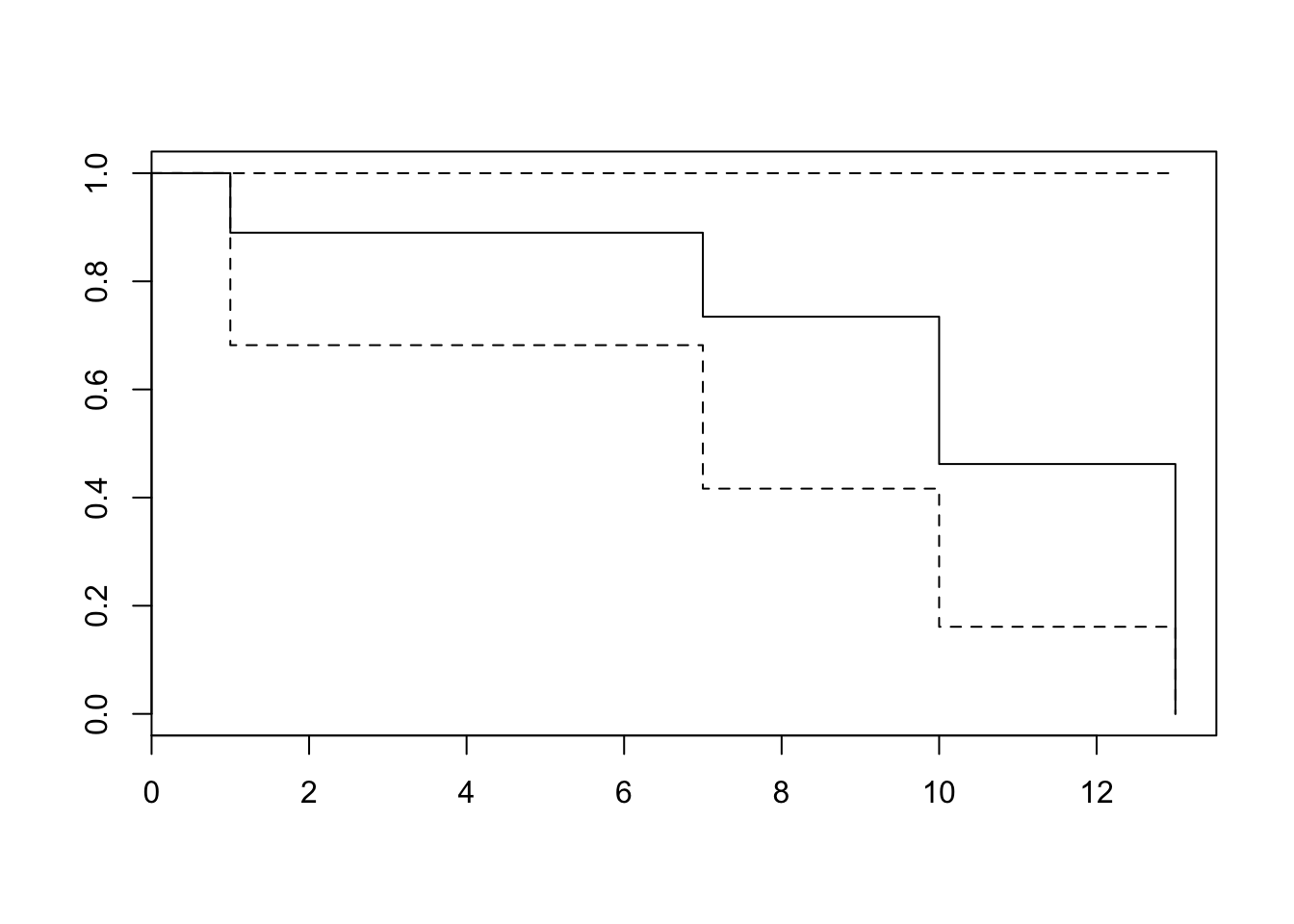
Note that the exp(coef) is the hazard ratio. When it is greater than 1, there is an increase in hazard, and when it is less than 1, there is a decrease in the hazard. We can do a test for proportional hazards as follows, and examine the p-values.
cox.zph(res)## rho chisq p
## female 0.563 1.504 0.220
## age -0.472 0.743 0.389
## GLOBAL NA 1.762 0.414Finally, we are interested in obtaining the baseline hazard function \(\lambda_0(t)\) which as we know has dropped out of the estimation. So how do we recover it? In fact, without it, where do we even get \(\lambda_i(t)\) from? We would also like to get the cumulative baseline hazard, i.e., \(\Lambda_0(t) = \int_0^t \lambda_0(u) du\). Sadly, this is a major deficiency of the Cox PH model. However, one may make a distributional assumption about the form of \(\lambda_0(t)\) and then fit it to maximize the likelihood of survival times, after the coefficients \(\beta\) have been fit already. For example, one function might be \(\lambda_0(t) = e^{\alpha t}\), and it would only need the estimation of \(\alpha\). We can then obtain the estimated survival probabilities over time.
covs <- data.frame(age = 21, female = 0)
summary(survfit(res, newdata = covs, type = "aalen"))
## Call: survfit(formula = res, newdata = covs, type = "aalen")
##
## time n.risk n.event survival std.err lower 95% CI upper 95% CI
## 1 6 1 0.9475 0.108 7.58e-01 1
## 7 4 1 0.8672 0.236 5.08e-01 1
## 10 3 1 0.7000 0.394 2.32e-01 1
## 13 1 1 0.0184 0.117 7.14e-08 1The “survival” column gives the survival probabilty for various time horizons shown in the first column.
For a useful guide, see https://rpubs.com/daspringate/survival
To sum up, see that the Cox PH model estimates the hazard rate function (t):
\[ \lambda(t) = \lambda_0(t) \exp[\beta^\top x] \]
The “exp(coef)” is the baseline hazard rate multiplier effect. If exp(coef)>1, then an increase in the variable \(x\) increases the hazard rate by that factor, and if exp(coef)<1, then it reduces the hazard rate \(\lambda(t)\) by that factor. Note that the hazard rate is NOT the probability of survival, and in fact \(\lambda(t) \in (0,\infty)\). Note that the probability of survival over time t, if we assume a constant hazard rate \(\lambda\) is \(s(t) = e^{-\lambda t}\). Of course \(s(t) \in (0,1)\).
So for example, if the current (assumed constant) hazard rate is \(\lambda = 0.02\), then the (for example) 3-year survival probability is
\[ s(t) = e^{-0.02 \times 3} = 0.9418 \]
If the person is female, then the new hazard rate is \(\lambda \times 4.686 = 0.09372\). So the new survival probability is
\[ s(t=3) = e^{-0.09372 \times 3} = 0.7549 \]
If Age increases by one year then the new hazard rate will be \(0.02 \times 0.3886 = 0.007772\). And the new survival probability will be
\[ s(t=3) = e^{-0.007772 \times 3} = 0.977 \]
Note that the hazard rate and the probability of survival go in opposite directions.
11.17 GLMNET: Lasso and Ridge Regressions
The glmnet package is from Stanford, and you can get all the details and examples here: https://web.stanford.edu/~hastie/glmnet/glmnet_alpha.html
The package fits generalized linear models and also penalizes the size of the model, with various standard models as special cases.
The function equation for minimization is
\[ \min_{\beta} \frac{1}{n}\sum_{i=1}^n w_i L(y_i,\beta^\top x_i) + \lambda \left[(1-\alpha) \frac{1}{2}\| \beta \|_2^2 + \alpha \|\beta \|_1\right] \]
where \(\|\beta\|_1\) and \(\|\beta\|_2\) are the \(L_1\) and \(L_2\) norms for tge vector \(\beta\). The idea is to take any loss function and penalize it. For example, if the loss function is just the sum of squared residuals \(y_i-\beta^\top x_i\), and \(w_i=1, \lambda=0\), then we get an ordinary least squares regression model. The function \(L\) is usually set to be the log-likelihood function.
If the \(L_1\) norm is applied only, i.e., \(\alpha=1\), then we get the Lasso model. If the \(L_2\) norm is solely applied, i.e., \(\alpha=0\), then we get a ridge regression. As is obvious from the equation, \(\lambda\) is the size of the penalty applied, and increasing this parameter forces a more parsimonious model.
Here is an example of lasso (\(\alpha=1\)):
suppressMessages(library(glmnet))

ncaa = read.table("DSTMAA_data/ncaa.txt",header=TRUE)
y = c(rep(1,32),rep(0,32))
x = as.matrix(ncaa[4:14])
res = cv.glmnet(x = x, y = y, family = 'binomial', alpha = 1, type.measure = "auc")
## Warning: Too few (< 10) observations per fold for type.measure='auc' in
## cv.lognet; changed to type.measure='deviance'. Alternatively, use smaller
## value for nfoldsplot(res)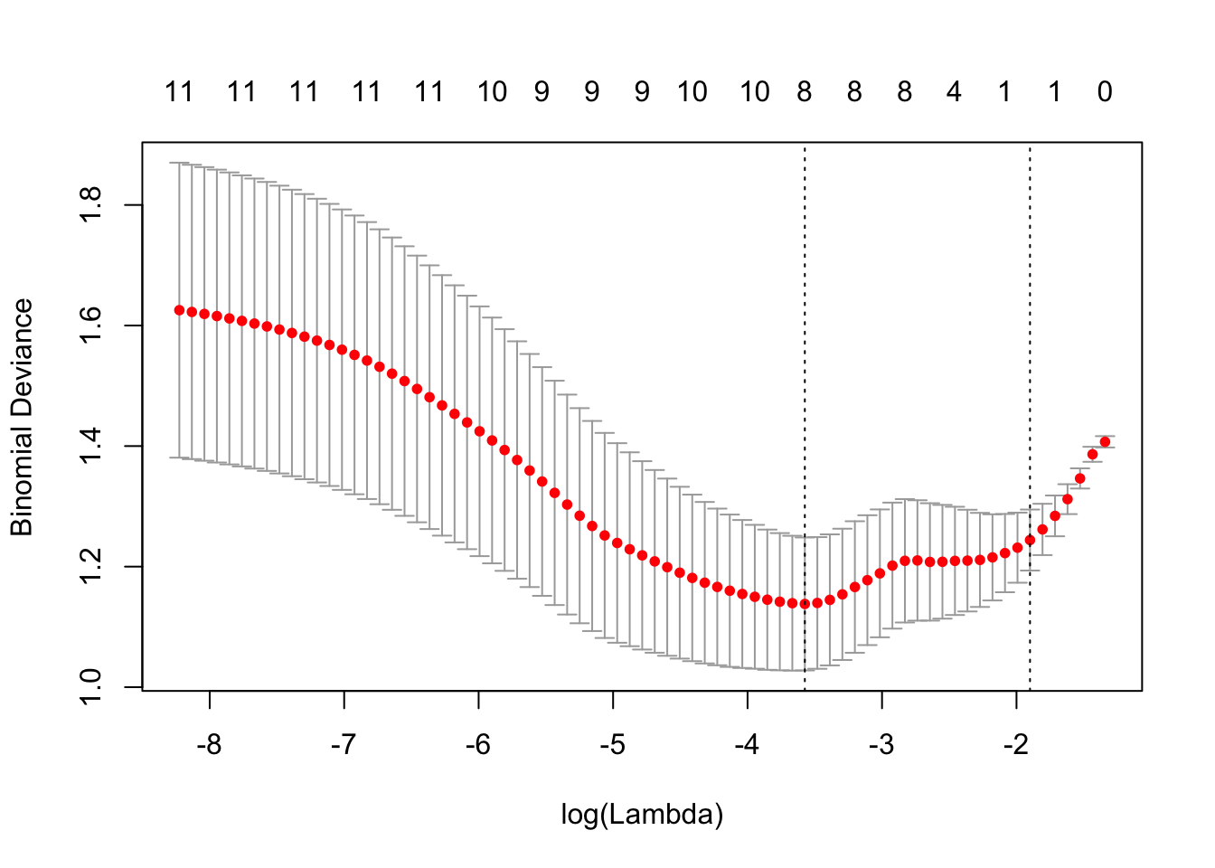
We may also run glmnet to get coefficients.
res = glmnet(x = x, y = y, family = 'binomial', alpha = 1)
print(names(res))
## [1] "a0" "beta" "df" "dim" "lambda"
## [6] "dev.ratio" "nulldev" "npasses" "jerr" "offset"
## [11] "classnames" "call" "nobs"print(res)##
## Call: glmnet(x = x, y = y, family = "binomial", alpha = 1)
##
## Df %Dev Lambda
## [1,] 0 1.602e-16 0.2615000
## [2,] 1 3.357e-02 0.2383000
## [3,] 1 6.172e-02 0.2171000
## [4,] 1 8.554e-02 0.1978000
## [5,] 1 1.058e-01 0.1803000
## [6,] 1 1.231e-01 0.1642000
## [7,] 1 1.380e-01 0.1496000
## [8,] 1 1.508e-01 0.1364000
## [9,] 1 1.618e-01 0.1242000
## [10,] 2 1.721e-01 0.1132000
## [11,] 4 1.851e-01 0.1031000
## [12,] 5 1.990e-01 0.0939800
## [13,] 4 2.153e-01 0.0856300
## [14,] 4 2.293e-01 0.0780300
## [15,] 4 2.415e-01 0.0711000
## [16,] 5 2.540e-01 0.0647800
## [17,] 8 2.730e-01 0.0590200
## [18,] 8 2.994e-01 0.0537800
## [19,] 8 3.225e-01 0.0490000
## [20,] 8 3.428e-01 0.0446500
## [21,] 8 3.608e-01 0.0406800
## [22,] 8 3.766e-01 0.0370700
## [23,] 8 3.908e-01 0.0337800
## [24,] 8 4.033e-01 0.0307800
## [25,] 8 4.145e-01 0.0280400
## [26,] 9 4.252e-01 0.0255500
## [27,] 10 4.356e-01 0.0232800
## [28,] 10 4.450e-01 0.0212100
## [29,] 10 4.534e-01 0.0193300
## [30,] 10 4.609e-01 0.0176100
## [31,] 10 4.676e-01 0.0160500
## [32,] 10 4.735e-01 0.0146200
## [33,] 10 4.789e-01 0.0133200
## [34,] 10 4.836e-01 0.0121400
## [35,] 10 4.878e-01 0.0110600
## [36,] 9 4.912e-01 0.0100800
## [37,] 9 4.938e-01 0.0091820
## [38,] 9 4.963e-01 0.0083670
## [39,] 9 4.984e-01 0.0076230
## [40,] 9 5.002e-01 0.0069460
## [41,] 9 5.018e-01 0.0063290
## [42,] 9 5.032e-01 0.0057670
## [43,] 9 5.044e-01 0.0052540
## [44,] 9 5.055e-01 0.0047880
## [45,] 9 5.064e-01 0.0043620
## [46,] 9 5.071e-01 0.0039750
## [47,] 10 5.084e-01 0.0036220
## [48,] 10 5.095e-01 0.0033000
## [49,] 10 5.105e-01 0.0030070
## [50,] 10 5.114e-01 0.0027400
## [51,] 10 5.121e-01 0.0024960
## [52,] 10 5.127e-01 0.0022750
## [53,] 11 5.133e-01 0.0020720
## [54,] 11 5.138e-01 0.0018880
## [55,] 11 5.142e-01 0.0017210
## [56,] 11 5.146e-01 0.0015680
## [57,] 11 5.149e-01 0.0014280
## [58,] 11 5.152e-01 0.0013020
## [59,] 11 5.154e-01 0.0011860
## [60,] 11 5.156e-01 0.0010810
## [61,] 11 5.157e-01 0.0009846
## [62,] 11 5.158e-01 0.0008971
## [63,] 11 5.160e-01 0.0008174
## [64,] 11 5.160e-01 0.0007448
## [65,] 11 5.161e-01 0.0006786
## [66,] 11 5.162e-01 0.0006183
## [67,] 11 5.162e-01 0.0005634
## [68,] 11 5.163e-01 0.0005134
## [69,] 11 5.163e-01 0.0004678
## [70,] 11 5.164e-01 0.0004262
## [71,] 11 5.164e-01 0.0003883
## [72,] 11 5.164e-01 0.0003538
## [73,] 11 5.164e-01 0.0003224
## [74,] 11 5.164e-01 0.0002938
## [75,] 11 5.165e-01 0.0002677
## [76,] 11 5.165e-01 0.0002439
## [77,] 11 5.165e-01 0.0002222b = coef(res)[,25] #Choose the best case with 8 coefficients
print(b)## (Intercept) PTS REB AST TO
## -17.30807199 0.04224762 0.13304541 0.00000000 -0.13440922
## A.T STL BLK PF FG
## 0.63059336 0.21867734 0.11635708 0.00000000 17.14864201
## FT X3P
## 3.00069901 0.00000000x1 = c(1,as.numeric(x[18,]))
p = 1/(1+exp(-sum(b*x1)))
print(p)## [1] 0.769648111.17.1 Prediction on test data
preds = predict(res, x, type = 'response')
print(dim(preds))
## [1] 64 77preds = preds[,25] #Take the 25th case
print(preds)## [1] 0.97443940 0.90157397 0.87711437 0.89911656 0.95684199 0.82949042
## [7] 0.53186622 0.83745812 0.45979765 0.58355756 0.78726183 0.55050365
## [13] 0.30633472 0.93605170 0.70646742 0.85811465 0.42394178 0.76964806
## [19] 0.40172414 0.66137964 0.69620096 0.61569705 0.88800581 0.92834645
## [25] 0.82719624 0.17209046 0.66881541 0.84149477 0.58937886 0.64674446
## [31] 0.79368965 0.51186217 0.58500925 0.61275721 0.17532362 0.47406867
## [37] 0.24314471 0.11843924 0.26787937 0.24296988 0.21129918 0.05041436
## [43] 0.30109650 0.14989973 0.17976216 0.57119150 0.05514704 0.46220128
## [49] 0.63788393 0.32605605 0.35544396 0.12647374 0.61772958 0.63883954
## [55] 0.02306762 0.21285032 0.36455131 0.53953727 0.18563868 0.23598354
## [61] 0.11821886 0.04258418 0.19603015 0.24630145print(glmnet:::auc(y, preds))## [1] 0.9072266print(table(y,round(preds,0))) #rounding needed to make 0,1##
## y 0 1
## 0 25 7
## 1 5 2711.18 ROC Curves
ROC stands for Receiver Operating Characteristic. The acronym comes from signal theory, where the users are interested in the number of true positive signals that are identified. The idea is simple, and best explained with an example. Let’s say you have an algorithm that detects customers probability \(p \in (0,1)\) of buying a product. Take a tagged set of training data and sort the customers by this probability in a line with the highest propensity to buy on the left and moving to the right the probabilty declines monotonically. (Tagged means you know whether they bought the product or not.) Now, starting from the left, plot a line that jumps vertically by a unit if the customer buys the product as you move across else remains flat. If the algorithm is a good one, the line will quickly move up at first and then flatten out.
Let’s take the train and test data here and plot the ROC curve by writing our own code.
We can do the same with the pROC package. Here is the code.
suppressMessages(library(pROC))## Warning: package 'pROC' was built under R version 3.3.2res = roc(response=y,predictor=preds)
print(res)##
## Call:
## roc.default(response = y, predictor = preds)
##
## Data: preds in 32 controls (y 0) < 32 cases (y 1).
## Area under the curve: 0.9072plot(res); grid()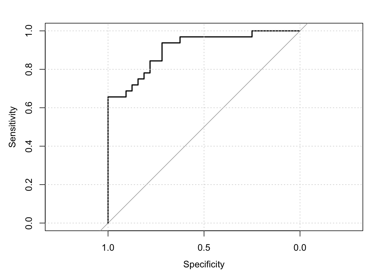
We see that “specificity” equals the true negative rate, and is also denoted as “recall”. And that the true positive rate is also labeled as “sensitivity”. The AUC or “area under the curve”" is the area between the curve and the diagonal divided by the area in the top right triangle of the diagram. This is also reported and is the same number as obtained when we fitted the model using the glmnet function before. For nice graphics that explain all these measures and more, see https://en.wikipedia.org/wiki/Precision_and_recall
11.19 Glmnet Cox Models
As we did before, we may fit a Cox PH model using GLMNET with the additional feature that we include a penalty when we maximize the likelihood function.
SURV = read.table("DSTMAA_data/survival_data.txt",header=TRUE)
print(SURV)
## id time death age female
## 1 1 1 1 20 0
## 2 2 4 0 21 1
## 3 3 7 1 19 0
## 4 4 10 1 22 1
## 5 5 12 0 20 0
## 6 6 13 1 24 1names(SURV)[3] = "status"
y = as.matrix(SURV[,2:3])
x = as.matrix(SURV[,4:5])
res = glmnet(x, y, family = "cox")
print(res)##
## Call: glmnet(x = x, y = y, family = "cox")
##
## Df %Dev Lambda
## [1,] 0 0.00000 0.331700
## [2,] 1 0.02347 0.302200
## [3,] 1 0.04337 0.275400
## [4,] 1 0.06027 0.250900
## [5,] 1 0.07466 0.228600
## [6,] 1 0.08690 0.208300
## [7,] 1 0.09734 0.189800
## [8,] 1 0.10620 0.172900
## [9,] 1 0.11380 0.157600
## [10,] 1 0.12020 0.143600
## [11,] 1 0.12570 0.130800
## [12,] 1 0.13040 0.119200
## [13,] 1 0.13430 0.108600
## [14,] 1 0.13770 0.098970
## [15,] 1 0.14050 0.090180
## [16,] 1 0.14300 0.082170
## [17,] 1 0.14500 0.074870
## [18,] 1 0.14670 0.068210
## [19,] 1 0.14820 0.062150
## [20,] 1 0.14940 0.056630
## [21,] 1 0.15040 0.051600
## [22,] 1 0.15130 0.047020
## [23,] 1 0.15200 0.042840
## [24,] 1 0.15260 0.039040
## [25,] 1 0.15310 0.035570
## [26,] 2 0.15930 0.032410
## [27,] 2 0.16480 0.029530
## [28,] 2 0.16930 0.026910
## [29,] 2 0.17320 0.024520
## [30,] 2 0.17640 0.022340
## [31,] 2 0.17910 0.020350
## [32,] 2 0.18140 0.018540
## [33,] 2 0.18330 0.016900
## [34,] 2 0.18490 0.015400
## [35,] 2 0.18630 0.014030
## [36,] 2 0.18740 0.012780
## [37,] 2 0.18830 0.011650
## [38,] 2 0.18910 0.010610
## [39,] 2 0.18980 0.009669
## [40,] 2 0.19030 0.008810
## [41,] 2 0.19080 0.008028
## [42,] 2 0.19120 0.007314
## [43,] 2 0.19150 0.006665
## [44,] 2 0.19180 0.006073
## [45,] 2 0.19200 0.005533
## [46,] 2 0.19220 0.005042
## [47,] 2 0.19240 0.004594
## [48,] 2 0.19250 0.004186
## [49,] 2 0.19260 0.003814
## [50,] 2 0.19270 0.003475
## [51,] 2 0.19280 0.003166
## [52,] 2 0.19280 0.002885
## [53,] 2 0.19290 0.002629
## [54,] 2 0.19290 0.002395
## [55,] 2 0.19300 0.002182
## [56,] 2 0.19300 0.001988plot(res)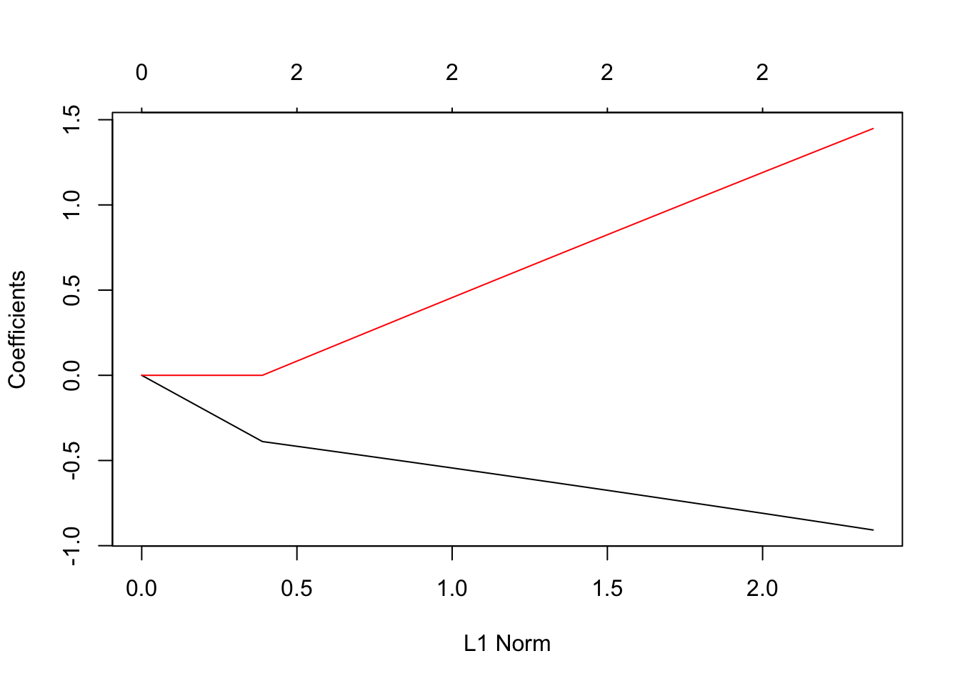
print(coef(res))## 2 x 56 sparse Matrix of class "dgCMatrix"## [[ suppressing 56 column names 's0', 's1', 's2' ... ]]##
## age . -0.03232796 -0.06240328 -0.09044971 -0.1166396 -0.1411157
## female . . . . . .
##
## age -0.1639991 -0.185342 -0.2053471 -0.2240373 -0.2414872 -0.2577658
## female . . . . . .
##
## age -0.272938 -0.2870651 -0.3002053 -0.3124148 -0.3237473 -0.3342545
## female . . . . . .
##
## age -0.3440275 -0.3530249 -0.3613422 -0.3690231 -0.3761098 -0.3826423
## female . . . . . .
##
## age -0.3886591 -0.4300447 -0.4704889 -0.5078614 -0.5424838 -0.5745449
## female . 0.1232263 0.2429576 0.3522138 0.4522592 0.5439278
##
## age -0.6042077 -0.6316057 -0.6569988 -0.6804703 -0.7022042 -0.7222141
## female 0.6279337 0.7048655 0.7754539 0.8403575 0.9000510 0.9546989
##
## age -0.7407295 -0.7577467 -0.773467 -0.7878944 -0.8012225 -0.8133071
## female 1.0049765 1.0509715 1.093264 1.1319284 1.1675026 1.1999905
##
## age -0.8246563 -0.8349496 -0.8442393 -0.8528942 -0.860838 -0.8680639
## female 1.2297716 1.2570025 1.2817654 1.3045389 1.325398 1.3443458
##
## age -0.874736 -0.8808466 -0.8863844 -0.8915045 -0.8961894 -0.9004172
## female 1.361801 1.3777603 1.3922138 1.4055495 1.4177359 1.4287319
##
## age -0.9043351 -0.9079181
## female 1.4389022 1.4481934With cross validation, we get the usual plot for the fit.
cvfit = cv.glmnet(x, y, family = "cox")
plot(cvfit)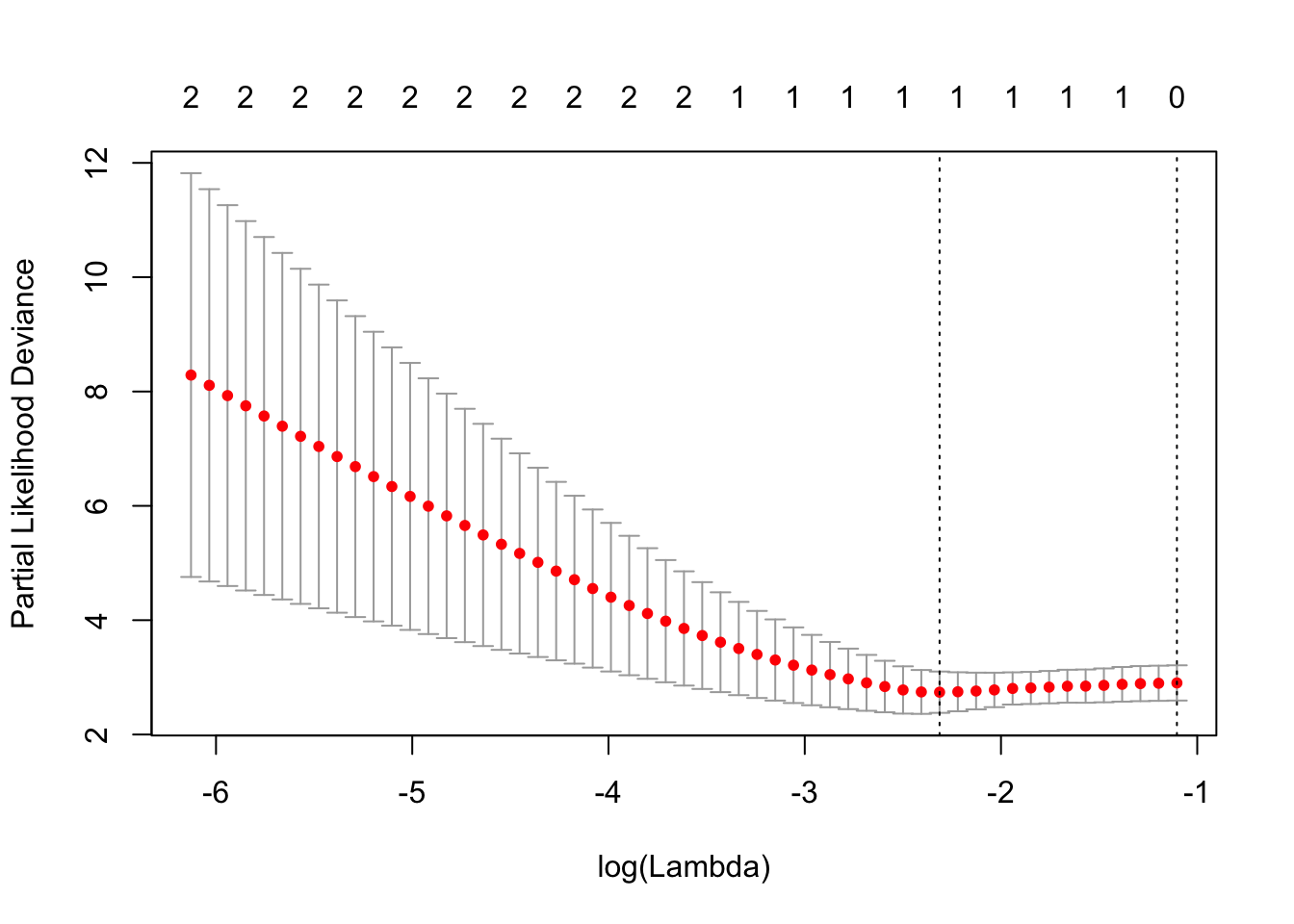
print(cvfit$lambda.min)## [1] 0.0989681print(coef(cvfit,s=cvfit$lambda.min))## 2 x 1 sparse Matrix of class "dgCMatrix"
## 1
## age -0.2870651
## female .Note that the signs of the coefficients are the same as we had earlier, i.e., survival is lower with age and higher for females.
References
Brander, James A., Raphael Amit, and Werner Antweiler. 2002. “Venture-Capital Syndication: Improved Venture Selection Vs. the Value-Added Hypothesis.” Journal of Economics & Management Strategy 11 (3). Blackwell Publishing Ltd.: 423–52. doi:10.1111/j.1430-9134.2002.00423.x.
Lerner, Joshua. 1994. “The Syndication of Venture Capital Investments.” Financial Management 23 (3). [Financial Management Association International, Wiley]: 16–27. http://www.jstor.org/stable/3665618.