Chapter 13 Statistical Brains: Neural Networks
13.1 Overview
Neural networks are special forms of nonlinear regressions where the decision system for which the NN is built mimics the way the brain is supposed to work (whether it works like a NN is up for grabs of course).
Terrific online book: http://neuralnetworksanddeeplearning.com/
13.2 Perceptrons
The basic building block of a neural network is a perceptron. A perceptron is like a neuron in a human brain. It takes inputs (e.g. sensory in a real brain) and then produces an output signal. An entire network of perceptrons is called a neural net.
For example, if you make a credit card application, then the inputs comprise a whole set of personal data such as age, sex, income, credit score, employment status, etc, which are then passed to a series of perceptrons in parallel. This is the first layer of assessment. Each of the perceptrons then emits an output signal which may then be passed to another layer of perceptrons, who again produce another signal. This second layer is often known as the hidden perceptron layer. Finally, after many hidden layers, the signals are all passed to a single perceptron which emits the decision signal to issue you a credit card or to deny your application.
Perceptrons may emit continuous signals or binary \((0,1)\) signals. In the case of the credit card application, the final perceptron is a binary one. Such perceptrons are implemented by means of squashing functions. For example, a really simple squashing function is one that issues a 1 if the function value is positive and a 0 if it is negative. More generally,
\[\begin{equation} S(x) = \left\{ \begin{array}{cl} 1 & \mbox{if } g(x)>T \\ 0 & \mbox{if } g(x) \leq T \end{array} \right. \end{equation}\]where \(g(x)\) is any function taking positive and negative values, for instance, \(g(x) \in (-\infty, +\infty)\). \(T\) is a threshold level.
A neural network with many layers is also known as a multi-layered perceptron, i.e., all those perceptrons together may be thought of as one single, big perceptron.
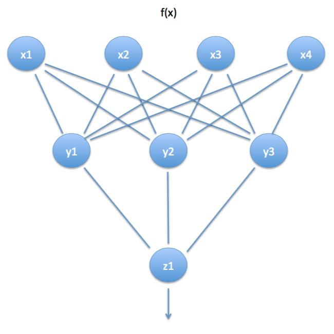
x is the input layer, y is the hidden layer, and z is the output layer.
13.3 Deep Learning
Neural net models are related to Deep Learning, where the number of hidden layers is vastly greater than was possible in the past when computational power was limited. Now, deep learning nets cascade through 20-30 layers, resulting in a surprising ability of neural nets in mimicking human learning processes. see: http://en.wikipedia.org/wiki/Deep_learning
And also see: http://deeplearning.net/
13.4 Binary NNs
Binary NNs are also thought of as a category of classifier systems. They are widely used to divide members of a population into classes. But NNs with continuous output are also popular. As we will see later, researchers have used NNs to learn the Black-Scholes option pricing model.
Areas of application: credit cards, risk management, forecasting corporate defaults, forecasting economic regimes, measuring the gains from mass mailings by mapping demographics to success rates.
13.5 Squashing Functions
Squashing functions may be more general than just binary. They usually squash the output signal into a narrow range, usually \((0,1)\). A common choice is the logistic function (also known as the sigmoid function).
\[\begin{equation} f(x) = \frac{1}{1+e^{-w\;x}} \end{equation}\]Think of \(w\) as the adjustable weight. Another common choice is the probit function
\[\begin{equation} f(x) = \Phi(w\;x) \end{equation}\]where \(\Phi(\cdot)\) is the cumulative normal distribution function.
13.6 How does the NN work?
The easiest way to see how a NN works is to think of the simplest NN, i.e. one with a single perceptron generating a binary output. The perceptron has \(n\) inputs, with values \(x_i, i=1...n\) and current weights \(w_i, i=1...n\). It generates an output \(y\).
The net input is defined as
\[\begin{equation} \sum_{i=1}^n w_i x_i \end{equation}\]If a function of the net input is greater than a threshold \(T\), then the output signal is \(y=1\), and if it is less than \(T\), the output is \(y=0\). The actual output is called the desired output and is denoted \(d = \{0,1\}\). Hence, the training data provided to the NN comprises both the inputs \(x_i\) and the desired output \(d\).
The output of our single perceptron model will be the sigmoid function of the net input, i.e.
\[\begin{equation} y = \frac{1}{1+\exp\left( - \sum_{i=1}^n w_i x_i \right)} \end{equation}\]For a given input set, the error in the NN is given by some loss function, an example of which is below:
\[\begin{equation} E = \frac{1}{2} \sum_{j=1}^m (y_j - d_j)^2 \end{equation}\]where \(m\) is the size of the training data set. The optimal NN for given data is obtained by finding the weights \(w_i\) that minimize this error function \(E\). Once we have the optimal weights, we have a calibrated feed-forward neural net.
For a given squashing function \(f\), and input \(x = [x_1, x_2, \ldots, x_n]'\), the multi-layer perceptron will given an output at each node of the hidden layer of
\[\begin{equation} y(x) = f \left(w_0 + \sum_{j=1}^n w_j x_j \right) \end{equation}\]and then at the final output level the node is
\[\begin{equation} z(x) = f\left( w_0 + \sum_{i=1}^N w_i \cdot f \left(w_{0i} + \sum_{j=1}^n w_{ji} x_j \right) \right) \end{equation}\]where the nested structure of the neural net is quite apparent. The \(f\) functions are also known as activation functions.
13.7 Relationship to Logit/Probit Models
The special model above with a single perceptron is actually nothing else than the logit regression model. If the squashing function is taken to the cumulative normal distribution, then the model becomes the probit regression model. In both cases though, the model is fitted by minimizing squared errors, not by maximum likelihood, which is how standard logit/probit models are parameterized.
13.8 Connection to hyperplanes
Note that in binary squashing functions, the net input is passed through a sigmoid function and then compared to the threshold level \(T\). This sigmoid function is a monotone one. Hence, this means that there must be a level \(T'\) at which the net input \(\sum_{i=1}^n w_i x_i\) must be for the result to be on the cusp. The following is the equation for a hyperplane
\[\begin{equation} \sum_{i=1}^n w_i x_i = T' \end{equation}\]which also implies that observations in \(n\)-dimensional space of the inputs \(x_i\), must lie on one side or the other of this hyperplane. If above the hyperplane, then \(y=1\), else \(y=0\). Hence, single perceptrons in neural nets have a simple geometrical intuition.
13.9 Gradient Descent
We start with a simple function. We want to minimize this function. But let’s plot it first to see where the minimum lies.
f = function(x) { result = 3*x^2 - 5*x + 10 }
x = seq(-4,4,0.1)
plot(x,f(x),type="l")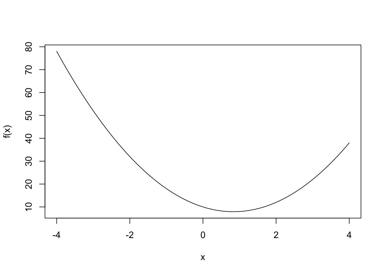
Next, we solve for \(x_{min}\), the value at which the function is minimized, which appears to lie between \(0\) and \(2\). We do this by gradient descent, from an initial value for \(x=-3\). We then run down the function to its minimum but manage the rate of descent using a paramater \(\eta=0.10\). The evolution (descent) equation is called recursively through the following dynamics for \(x\):
\[ x \leftarrow x - \eta \cdot \frac{\partial f}{\partial x} \]
If the gradient is positive, then we need to head in the opposite direction to reach the minimum, and hence, we have a negative sign in front of the modification term above. But first we need to calculate the gradient, and the descent. To repeat, first gradient, then descent!
x = -3
eta = 0.10
dx = 0.0001
grad = (f(x+dx)-f(x))/dx
x = x - eta*grad
print(x)
## [1] -0.70003We see that \(x\) has moved closer to the value that minimizes the function. We can repeat thismany times till it settles down at the minimum, each round of updates being called an epoch. We run 20 epochs next.
for (j in 1:20) {
  grad = (f(x+dx)-f(x))/dx
  x = x - eta*grad
  print(c(j,x,grad,f(x)))
}
## [1] 1.000000 0.219958 -9.199880 9.045355
## [1] 2.0000000 0.5879532 -3.6799520 8.0973009
## [1] 3.0000000 0.7351513 -1.4719808 7.9455858
## [1] 4.0000000 0.7940305 -0.5887923 7.9213008
## [1] 5.0000000 0.8175822 -0.2355169 7.9174110
## [1] 6.00000000 0.82700288 -0.09420677 7.91678689
## [1] 7.00000000 0.83077115 -0.03768271 7.91668636
## [1] 8.00000000 0.83227846 -0.01507308 7.91667000
## [1] 9.000000000 0.832881384 -0.006029233 7.916667279
## [1] 10.000000000 0.833122554 -0.002411693 7.916666800
## [1] 11.0000000000 0.8332190215 -0.0009646773 7.9166667059
## [1] 12.0000000000 0.8332576086 -0.0003858709 7.9166666839
## [1] 13.0000000000 0.8332730434 -0.0001543484 7.9166666776
## [1] 1.400000e+01 8.332792e-01 -6.173935e-05 7.916667e+00
## [1] 1.500000e+01 8.332817e-01 -2.469573e-05 7.916667e+00
## [1] 1.600000e+01 8.332827e-01 -9.878303e-06 7.916667e+00
## [1] 1.700000e+01 8.332831e-01 -3.951310e-06 7.916667e+00
## [1] 1.800000e+01 8.332832e-01 -1.580540e-06 7.916667e+00
## [1] 1.900000e+01 8.332833e-01 -6.322054e-07 7.916667e+00
## [1] 2.000000e+01 8.332833e-01 -2.528822e-07 7.916667e+00It has converged really quickly! At convergence, the gradient goes to zero.
13.10 Feedback and Backpropagation
What distinguishes neural nets from ordinary nonlinear regressions is feedback. Neural nets learn from feedback as they are used. Feedback is implemented using a technique called backpropagation.
Suppose you have a calibrated NN. Now you obtain another observation of data and run it through the NN. Comparing the output value \(y\) with the desired observation \(d\) gives you the error for this observation. If the error is large, then it makes sense to update the weights in the NN, so as to self-correct. This process of self-correction is known as gradient descent via backpropagation.
The benefit of gradient descent via backpropagation is that a full re-fitting exercise may not be required. Using simple rules the correction to the weights can be applied gradually in a learning manner.
Lets look at fitting with a simple example using a single perceptron. Consider the \(k\)-th perceptron. The sigmoid of this is
\[\begin{equation} y_k = \frac{1}{1+\exp\left( - \sum_{i=1}^n w_{i} x_{ik} \right)} \end{equation}\]where \(y_k\) is the output of the \(k\)-th perceptron, and \(x_{ik}\) is the \(i\)-th input to the \(k\)-th perceptron. The error from this observation is \((y_k - d_k)\). Recalling that \(E = \frac{1}{2} \sum_{j=1}^m (y_j - d_j)^2\), we may compute the change in error with respect to the \(j\)-th output, i.e.
\[\begin{equation} \frac{\partial E}{\partial y_j} = y_j - d_j, \quad \forall j \end{equation}\]Note also that
\[\begin{equation} \frac{dy_j}{dx_{ij}} = y_j (1-y_j) w_i \end{equation}\]and
\[\begin{equation} \frac{dy_j}{dw_i} = y_j (1-y_j) x_{ij} \end{equation}\]Next, we examine how the error changes with input values:
\[\begin{equation} \frac{\partial E}{\partial x_{ij}} = \frac{\partial E}{\partial y_j} \times \frac{dy_j}{dx_{ij}} = (y_j - d_j) y_j (1-y_j) w_i \end{equation}\]We can now get to the value of interest, which is the change in error value with respect to the weights
\[\begin{equation} \frac{\partial E}{\partial w_{i}} = \frac{\partial E}{\partial y_j} \times \frac{dy_j}{dw_i} = (y_j - d_j)y_j (1-y_j) x_{ij}, \forall i \end{equation}\]We thus have one equation for each weight \(w_i\) and each observation \(j\). (Note that the \(w_i\) apply across perceptrons. A more general case might be where we have weights for each perceptron, i.e., \(w_{ij}\).) Instead of updating on just one observation, we might want to do this for many observations in which case the error derivative would be
\[\begin{equation} \frac{\partial E}{\partial w_{i}} = \sum_j (y_j - d_j)y_j (1-y_j) x_{ij}, \forall i \end{equation}\]Therefore, if \(\frac{\partial E}{\partial w_{i}} > 0\), then we would need to reduce \(w_i\) to bring down \(E\). By how much? Here is where some art and judgment is imposed. There is a tuning parameter \(0<\gamma<1\) which we apply to \(w_i\) to shrink it when the weight needs to be reduced. Likewise, if the derivative \(\frac{\partial E}{\partial w_{i}} < 0\), then we would increase \(w_i\) by dividing it by \(\gamma\). This is known as gradient descent.
13.11 Backpropagation
13.11.1 Extension to many observations
Our notation now becomes extended to weights \(w_{ik}\) which stand for the weight on the \(i\)-th input to the \(k\)-th perceptron. The derivative for the error becomes, across all observations \(j\):
\[\begin{equation} \frac{\partial E}{\partial w_{ik}} = \sum_j (y_j - d_j)y_j (1-y_j) x_{ikj}, \forall i,k \end{equation}\]Hence all nodes in the network have their weights updated. In many cases of course, we can just take the derivatives numerically. Change the weight \(w_{ik}\) and see what happens to the error.
However, the formal process of finding all the gradients using a fast algorithm via backpropagation requires more formal calculus, and the rest of this section provides detailed analysis showing how this is done.
13.12 Backprop: Detailed Analysis
In this section, we dig deeper into the incredible algebra that drives the unreasonable effectiveness of deep learning algorithms. To do this, we will work with a richer algebra, and extended notation.
13.12.1 Net Input
Assume several hidden layers in a deep learning net (DLN), indexed by \(r=1,2,...,R\). Consider two adjacent layers \((r)\) and \((r+1)\). Each layer as number of nodes \(n_r\) and \(n_{r+1}\), respectively.
The output of node \(i\) in layer \((r)\) is \(Z_i^{(r)} = f(a_i^{(r)})\). The function \(f\) is the activation function. At node \(j\) in layer \((r+1)\), these inputs are taken and used to compute an intermediate value, known as the net value:
\[ a_j^{(r+1)} = \sum_{i=1}^{n_r} W_{ij}^{(r+1)}Z_i^{r} + b_j^{(r+1)} \]
13.12.2 Activation Function
The net value is then ingested by an activation function to create the output from layer \((r+1)\).
\[ Z_j^{(r+1)} = f(a_j^{(r+1)}) \]
The activation functions may be simple sigmoid functions or other functions such as ReLU (Rectified Linear Unit). The final output of the DLN is from layer \((R)\), i.e., \(Z_j^{(R)}\).
For the first hidden layer \(r=1\), and the net input will be based on the original data \(X^{(m)}\)
\[ a_j^{(1)} = \sum_{m=1}^M W_{mj}^{(1)} X_m + b_j^{(1)} \]
13.12.3 Loss Function
Fitting the DLN is an exercise where the best weights \(\{W,b\} = \{W_{ij}^{(r+1)}, b_j^{(r+1)}\},\forall r\) for all layers are determined to minimize a loss function generally denoted as
\[ \min_{W,b} \sum_{m=1}^M L_m[h(X^{(m)}),T^{(m)}] \]
where \(M\) is the number of training observations (rows in the data set), \(T^{(m)}\) is the true value of the output, and \(h(X^{(m)})\) is the model output from the DLN. The loss function \(L_m\) quantifies the difference between the model output and the true output.
13.12.4 Gradients
To solve this minimization problem, we need gradients for all \(W,b\). These are denoted as
\[ \frac{\partial L_m}{\partial W_{ij}^{(r+1)}}, \quad \frac{\partial L_m}{\partial b_{j}^{(r+1)}}, \quad \forall r+1, j \]
We write out these gradients using the chain rule:
\[ \frac{\partial L_m}{\partial W_{ij}^{(r+1)}} = \frac{\partial L_m}{\partial a_j^{(r+1)}} \cdot \frac{\partial a_j^{(r+1)}}{\partial W_{ij}^{(r+1)}} = \delta_j^{(r+1)} \cdot Z_i^{(r)} \]
where we have written
\[ \delta_j^{(r+1)} = \frac{\partial L_m}{\partial a_j^{(r+1)}} \]
Likewise, we have
\[ \frac{\partial L_m}{\partial b_{j}^{(r+1)}} = \frac{\partial L_m}{\partial a_j^{(r+1)}} \cdot \frac{\partial a_j^{(r+1)}}{\partial b_{j}^{(r+1)}} = \delta_j^{(r+1)} \cdot 1 = \delta_j^{(r+1)} \]
13.12.5 Delta Values
So we need to find all the \(\delta_j^{(r+1)}\) values. To do so, we need the following intermediate calculation.
\[ \begin{align} a_j^{(r+1)} &= \sum_{i=1}^{n_r} W_{ij}^{(r+1)} Z_i^{(r)} + b_j^{(r+1)} \\ &= \sum_{i=1}^{n_r} W_{ij}^{(r+1)} f(a_i^{(r)}) + b_j^{(r+1)} \\ \end{align} \]
This implies that
\[ \frac{\partial a_j^{(r+1)}}{\partial a_i^{(r)}} = W_{ij}^{(r+1)} \cdot f'(a_i^{(r)}) \]
Using this we may now rewrite the \(\delta\) value for layer \((r)\) as follows:
\[ \begin{align} \delta_i^{(r)} &= \frac{\partial L_m}{\partial a_i^{(r)}} \\ &= \sum_{j=1}^{n_{r+1}} \frac{\partial L_m}{\partial a_j^{(r+1)}} \cdot \frac{\partial a_j^{(r+1)}}{\partial a_i^{(r)}} \\ &= \sum_{j=1}^{n_{r+1}}\delta_j^{(r+1)} \cdot W_{ij}^{(r+1)} \cdot f'(a_i^{(r)}) \\ &= f'(a_i^{(r)}) \cdot \sum_{j=1}^{n_{r+1}}\delta_j^{(r+1)} \cdot W_{ij}^{(r+1)} \end{align} \]
13.12.6 Output layer
The output layer takes as input the last hidden layer \({(R)}\)’s output \(Z_j^{(R)}\), and computes the net input \(a_j^{(R+1)}\) and then the activation function \(h(a_j^{(R+1)})\) is applied to generate the final output.
\[ \begin{align} a_j^{(R+1)} &= \sum_{i=1}^{n_R} W_{ij}^{(R+1)} Z_j^{(R)} + b_j^{(R+1)} \\ \mbox{Final output} &= h(a_j^{(R+1)}) \end{align} \]
The \(\delta\) for the final layer is simple.
\[ \delta_j^{(R+1)} = \frac{\partial L_m}{\partial a_j^{(R+1)}} = h'(a_j^{(R+1)}) \]
13.12.7 Feedforward and Backward Propagation
Fitting the DLN requires getting the weights \(\{W,b\}\) that minimize \(L_m\). These are done using gradient descent, i.e.,
\[ \begin{align} W_{ij}^{(r+1)} \leftarrow W_{ij}^{(r+1)} - \eta \cdot \frac{\partial L_m}{\partial W_{ij}^{(r+1)}} \\ b_{j}^{(r+1)} \leftarrow b_{j}^{(r+1)} - \eta \cdot \frac{\partial L_m}{\partial b_{j}^{(r+1)}} \end{align} \]
Here \(\eta\) is the learning rate parameter. We iterate on these functions until the gradients become zero, and the weights discontinue changing with each update, also known as an epoch.
The steps are as follows:
- Start with an initial set of weights \(\{w,b\}\).
- Feedforward the initial data and weights into the DLN, and find the \(\{a_i^{(r)}, Z_i^{(r)}\}, \forall r,i\). This is one forward pass through the network.
- Then, using backpropagation, compute all \(\delta_i^{(r)}, \forall r,i\).
- Use these \(\delta_i^{(r)}\) values to get all the new gradients.
- Apply gradient descent to get new weights.
- Keep iterating steps 2-5, until the chosen number of epochs is completed.
The entire process is summarized in Figure 13.1:
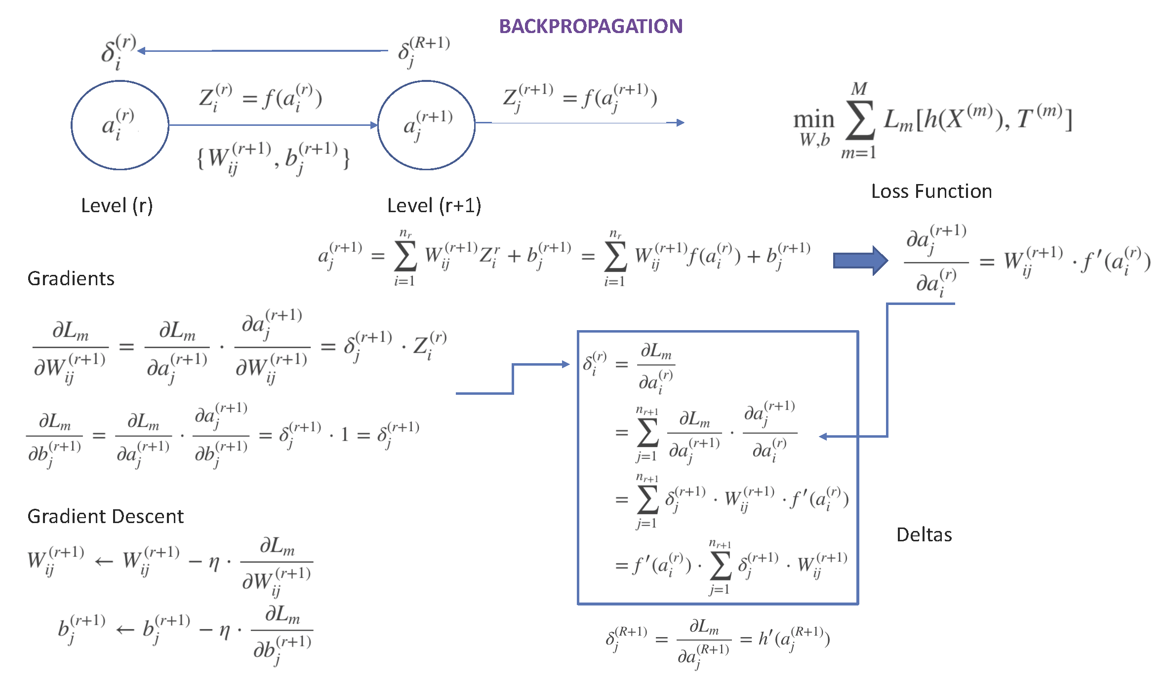
Figure 13.1: Quick Summary of Backpropagation
13.13 Research Applications
Discovering Black-Scholes: See the paper by Hutchinson, Lo, and Poggio (1994), A Nonparametric Approach to Pricing and Hedging Securities Via Learning Networks, The Journal of Finance, Vol XLIX.
Forecasting: See the paper by Ghiassi, Saidane, and Zimbra (2005). “A dynamic artificial neural network model for forecasting time series events,” International Journal of Forecasting 21, 341–362.
13.14 Package neuralnet in R
The package focuses on multi-layer perceptrons (MLP), see Bishop (1995), which are well applicable when modeling functional relation- ships. The underlying structure of an MLP is a directed graph, i.e. it consists of vertices and directed edges, in this context called neurons and synapses. See Bishop (1995), Neural networks for pattern recognition. Oxford University Press, New York.
The data set used by this package as an example is the infert data set that comes bundled with R.
This data set examines infertility after induced and spontaneous abortion. The variables induced and spontaneous take values in \(\{0,1,2\}\) indicating the number of previous abortions. The variable parity denotes the number of births. The variable case equals 1 if the woman is infertile and 0 otherwise. The idea is to model infertility.
library(neuralnet)
data(infert)
print(names(infert))
## [1] "education" "age" "parity" "induced"
## [5] "case" "spontaneous" "stratum" "pooled.stratum"head(infert)## education age parity induced case spontaneous stratum pooled.stratum
## 1 0-5yrs 26 6 1 1 2 1 3
## 2 0-5yrs 42 1 1 1 0 2 1
## 3 0-5yrs 39 6 2 1 0 3 4
## 4 0-5yrs 34 4 2 1 0 4 2
## 5 6-11yrs 35 3 1 1 1 5 32
## 6 6-11yrs 36 4 2 1 1 6 36summary(infert)## education age parity induced
## 0-5yrs : 12 Min. :21.00 Min. :1.000 Min. :0.0000
## 6-11yrs:120 1st Qu.:28.00 1st Qu.:1.000 1st Qu.:0.0000
## 12+ yrs:116 Median :31.00 Median :2.000 Median :0.0000
## Mean :31.50 Mean :2.093 Mean :0.5726
## 3rd Qu.:35.25 3rd Qu.:3.000 3rd Qu.:1.0000
## Max. :44.00 Max. :6.000 Max. :2.0000
## case spontaneous stratum pooled.stratum
## Min. :0.0000 Min. :0.0000 Min. : 1.00 Min. : 1.00
## 1st Qu.:0.0000 1st Qu.:0.0000 1st Qu.:21.00 1st Qu.:19.00
## Median :0.0000 Median :0.0000 Median :42.00 Median :36.00
## Mean :0.3347 Mean :0.5766 Mean :41.87 Mean :33.58
## 3rd Qu.:1.0000 3rd Qu.:1.0000 3rd Qu.:62.25 3rd Qu.:48.25
## Max. :1.0000 Max. :2.0000 Max. :83.00 Max. :63.00This data set examines infertility after induced and spontaneous abortion. The variables ** induced** and spontaneous take values in \(\{0,1,2\}\) indicating the number of previous abortions. The variable parity denotes the number of births. The variable case equals 1 if the woman is infertile and 0 otherwise. The idea is to model infertility.
13.14.1 First step, fit a logit model to the data.
res = glm(case ~ age+parity+induced+spontaneous, family=binomial(link="logit"), data=infert)
summary(res)
##
## Call:
## glm(formula = case ~ age + parity + induced + spontaneous, family = binomial(link = "logit"),
## data = infert)
##
## Deviance Residuals:
## Min 1Q Median 3Q Max
## -1.6281 -0.8055 -0.5299 0.8669 2.6141
##
## Coefficients:
## Estimate Std. Error z value Pr(>|z|)
## (Intercept) -2.85239 1.00428 -2.840 0.00451 **
## age 0.05318 0.03014 1.764 0.07767 .
## parity -0.70883 0.18091 -3.918 8.92e-05 ***
## induced 1.18966 0.28987 4.104 4.06e-05 ***
## spontaneous 1.92534 0.29863 6.447 1.14e-10 ***
## ---
## Signif. codes: 0 '***' 0.001 '**' 0.01 '*' 0.05 '.' 0.1 ' ' 1
##
## (Dispersion parameter for binomial family taken to be 1)
##
## Null deviance: 316.17 on 247 degrees of freedom
## Residual deviance: 260.94 on 243 degrees of freedom
## AIC: 270.94
##
## Number of Fisher Scoring iterations: 413.14.2 Second step, fit a NN
nn = neuralnet(case~age+parity+induced+spontaneous,hidden=2,data=infert)print(names(nn))## [1] "call" "response" "covariate"
## [4] "model.list" "err.fct" "act.fct"
## [7] "linear.output" "data" "net.result"
## [10] "weights" "startweights" "generalized.weights"
## [13] "result.matrix"nn$result.matrix## 1
## error 19.75482621709
## reached.threshold 0.00796839405
## steps 3891.00000000000
## Intercept.to.1layhid1 -2.39345712918
## age.to.1layhid1 -0.51858603247
## parity.to.1layhid1 0.26786607381
## induced.to.1layhid1 -346.33808632368
## spontaneous.to.1layhid1 6.50949229932
## Intercept.to.1layhid2 6.18035131278
## age.to.1layhid2 -0.13013668178
## parity.to.1layhid2 2.31764808626
## induced.to.1layhid2 -2.78558680449
## spontaneous.to.1layhid2 -4.58533007894
## Intercept.to.case 1.08152541274
## 1layhid.1.to.case -6.43770238799
## 1layhid.2.to.case -0.93730921525plot(nn)
#Run this plot from the command line.
#<img src="image_files/nn.png" height=510 width=740>head(cbind(nn$covariate,nn$net.result[[1]]))## [,1] [,2] [,3] [,4] [,5]
## 1 26 6 1 2 0.1522843862
## 2 42 1 1 0 0.5553601474
## 3 39 6 2 0 0.1442907090
## 4 34 4 2 0 0.1482055348
## 5 35 3 1 1 0.3599162573
## 6 36 4 2 1 0.474307288213.14.3 Logit vs NN
We can compare the output to that from the logit model, by looking at the correlation of the fitted values from both models.
cor(cbind(nn$net.result[[1]],res$fitted.values))## [,1] [,2]
## [1,] 1.0000000000 0.8869825759
## [2,] 0.8869825759 1.000000000013.14.4 Backpropagation option
We can add in an option for back propagation, and see how the results change.
nn2 = neuralnet(case~age+parity+induced+spontaneous,
             hidden=2, algorithm="rprop+", data=infert)
print(cor(cbind(nn2$net.result[[1]],res$fitted.values)))
## [,1] [,2]
## [1,] 1.0000000000 0.9157468405
## [2,] 0.9157468405 1.0000000000cor(cbind(nn2$net.result[[1]],nn$fitted.result[[1]]))## [,1]
## [1,] 1Given a calibrated neural net, how do we use it to compute values for a new observation? Here is an example.
compute(nn,covariate=matrix(c(30,1,0,1),1,4))## $neurons
## $neurons[[1]]
## [,1] [,2] [,3] [,4] [,5]
## [1,] 1 30 1 0 1
##
## $neurons[[2]]
## [,1] [,2] [,3]
## [1,] 1 0.00001403868578 0.5021422036
##
##
## $net.result
## [,1]
## [1,] 0.610772521113.15 Statistical Significance
We can assess statistical significance of the model as follows:
confidence.interval(nn,alpha=0.10)## $lower.ci
## $lower.ci[[1]]
## $lower.ci[[1]][[1]]
## [,1] [,2]
## [1,] -15.8007772276 4.3682646706
## [2,] -1.3384298107 -0.1876702868
## [3,] -0.2530961989 1.4895025332
## [4,] -346.3380863237 -3.6315599341
## [5,] -0.2056362177 -5.6749552264
##
## $lower.ci[[1]][[2]]
## [,1]
## [1,] 0.9354811195
## [2,] -38.0986993664
## [3,] -1.0879829307
##
##
##
## $upper.ci
## $upper.ci[[1]]
## $upper.ci[[1]][[1]]
## [,1] [,2]
## [1,] 11.0138629693 7.99243795495
## [2,] 0.3012577458 -0.07260307674
## [3,] 0.7888283465 3.14579363935
## [4,] -346.3380863237 -1.93961367486
## [5,] 13.2246208164 -3.49570493146
##
## $upper.ci[[1]][[2]]
##      [,1]
## [1,] 1.2275697059
## [2,] 25.2232945904
## [3,] -0.7866354998
##
##
##
## $nic
## [1] 21.21884675The confidence level is \((1-\alpha)\). This is at the 90% level, and at the 5% level we get:
confidence.interval(nn,alpha=0.95)## $lower.ci
## $lower.ci[[1]]
## $lower.ci[[1]][[1]]
## [,1] [,2]
## [1,] -2.9045845818 6.1112691082
## [2,] -0.5498409484 -0.1323300362
## [3,] 0.2480054218 2.2860766817
## [4,] -346.3380863237 -2.8178378500
## [5,] 6.2534913605 -4.6268698737
##
## $lower.ci[[1]][[2]]
## [,1]
## [1,] 1.0759577641
## [2,] -7.6447150209
## [3,] -0.9430533514
##
##
##
## $upper.ci
## $upper.ci[[1]]
## $upper.ci[[1]][[1]]
## [,1] [,2]
## [1,] -1.8823296766 6.2494335173
## [2,] -0.4873311166 -0.1279433273
## [3,] 0.2877267259 2.3492194908
## [4,] -346.3380863237 -2.7533357590
## [5,] 6.7654932382 -4.5437902841
##
## $upper.ci[[1]][[2]]
## [,1]
## [1,] 1.0870930614
## [2,] -5.2306897551
## [3,] -0.9315650791
##
##
##
## $nic
## [1] 21.2188467513.16 Deep Learning Overview
The Wikipedia entry is excellent: https://en.wikipedia.org/wiki/Deep_learning
https://www.youtube.com/watch?v=S75EdAcXHKk
https://www.youtube.com/watch?v=czLI3oLDe8M
Article on Google’s Deep Learning team’s work on image processing: https://medium.com/backchannel/inside-deep-dreams-how-google-made-its-computers-go-crazy-83b9d24e66df#.gtfwip891
13.16.1 Grab Some Data
The mlbench package contains some useful datasets for testing machine learning algorithms. One of these is a small dataset of cancer cases, and contains ten characteristics of cancer cells, and a flag for whether cancer is present or the cells are benign. We use this dataset to try out some deep learning algorithms in R, and see if they improve on vanilla neural nets. First, let’s fit a neural net to this data. We’ll fit this using the deepnet package, which allows for more hidden layers.
13.16.2 Simple Example
library(neuralnet)
library(deepnet)
First, we use randomly generated data, and train the NN.
#From the **deepnet** package by Xiao Rong. First train the model using one hidden layer.
Var1 <- c(rnorm(50, 1, 0.5), rnorm(50, -0.6, 0.2))
Var2 <- c(rnorm(50, -0.8, 0.2), rnorm(50, 2, 1))
x <- matrix(c(Var1, Var2), nrow = 100, ncol = 2)
y <- c(rep(1, 50), rep(0, 50))
plot(x,col=y+1)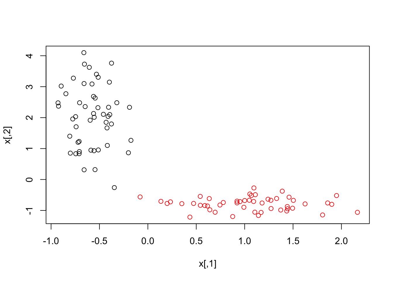
nn <- nn.train(x, y, hidden = c(5))13.16.3 Prediction
#Next, predict the model. This is in-sample.
test_Var1 <- c(rnorm(50, 1, 0.5), rnorm(50, -0.6, 0.2))
test_Var2 <- c(rnorm(50, -0.8, 0.2), rnorm(50, 2, 1))
test_x <- matrix(c(test_Var1, test_Var2), nrow = 100, ncol = 2)
yy <- nn.predict(nn, test_x)
13.16.4 Test Predictive Ability of the Model
#The output is just a number that is higher for one class and lower for another.
#One needs to separate these to get groups.
yhat = matrix(0,length(yy),1)
yhat[which(yy > mean(yy))] = 1
yhat[which(yy <= mean(yy))] = 0
print(table(yhat,y))
## y
## yhat 0 1
## 0 49 0
## 1 1 5013.16.5 Prediction Error
#Testing the results.
err <- nn.test(nn, test_x, y, t=mean(yy))
print(err)
## [1] 0.00513.17 Cancer dataset
Now we’ll try the Breast Cancer data set. First we use the NN in the deepnet package.
library(mlbench)
data("BreastCancer")
head(BreastCancer)
## Id Cl.thickness Cell.size Cell.shape Marg.adhesion Epith.c.size
## 1 1000025 5 1 1 1 2
## 2 1002945 5 4 4 5 7
## 3 1015425 3 1 1 1 2
## 4 1016277 6 8 8 1 3
## 5 1017023 4 1 1 3 2
## 6 1017122 8 10 10 8 7
## Bare.nuclei Bl.cromatin Normal.nucleoli Mitoses Class
## 1 1 3 1 1 benign
## 2 10 3 2 1 benign
## 3 2 3 1 1 benign
## 4 4 3 7 1 benign
## 5 1 3 1 1 benign
## 6 10 9 7 1 malignantBreastCancer = BreastCancer[which(complete.cases(BreastCancer)==TRUE),]y = as.matrix(BreastCancer[,11])
y[which(y=="benign")] = 0
y[which(y=="malignant")] = 1
y = as.numeric(y)
x = as.numeric(as.matrix(BreastCancer[,2:10]))
x = matrix(as.numeric(x),ncol=9)
nn <- nn.train(x, y, hidden = c(5))
yy = nn.predict(nn, x)
yhat = matrix(0,length(yy),1)
yhat[which(yy > mean(yy))] = 1
yhat[which(yy <= mean(yy))] = 0
print(table(y,yhat))## yhat
## y 0 1
## 0 424 20
## 1 5 23413.17.1 Compare to a simple NN
It does really well. Now we compare it to a simple neural net.
library(neuralnet)
df = data.frame(cbind(x,y))
nn = neuralnet(y~V1+V2+V3+V4+V5+V6+V7+V8+V9,data=df,hidden = 5)
yy = nn$net.result[[1]]
yhat = matrix(0,length(y),1)
yhat[which(yy > mean(yy))] = 1
yhat[which(yy <= mean(yy))] = 0
print(table(y,yhat))
## yhat
## y 0 1
## 0 429 15
## 1 0 239Somehow, the neuralnet package appears to perform better. Which is interesting. But the deep learning net was not “deep” - it had only one hidden layer.
13.19 Using h2o
Here we start up a server using all cores of the machine, and then use the h2o package’s deep learning toolkit to fit a model.
library(h2o)## Loading required package: methods## Loading required package: statmod## Warning: package 'statmod' was built under R version 3.3.2##
## ----------------------------------------------------------------------
##
## Your next step is to start H2O:
## > h2o.init()
##
## For H2O package documentation, ask for help:
## > ??h2o
##
## After starting H2O, you can use the Web UI at http://localhost:54321
## For more information visit http://docs.h2o.ai
##
## ----------------------------------------------------------------------##
## Attaching package: 'h2o'## The following objects are masked from 'package:stats':
##
## cor, sd, var## The following objects are masked from 'package:base':
##
## &&, %*%, %in%, ||, apply, as.factor, as.numeric, colnames,
## colnames<-, ifelse, is.character, is.factor, is.numeric, log,
## log10, log1p, log2, round, signif, trunclocalH2O = h2o.init(ip="localhost", port = 54321,
startH2O = TRUE, nthreads=-1)##
## H2O is not running yet, starting it now...
##
## Note: In case of errors look at the following log files:
## /var/folders/yd/h1lvwd952wbgw189srw3m3z80000gn/T//RtmpTFfRwJ/h2o_srdas_started_from_r.out
## /var/folders/yd/h1lvwd952wbgw189srw3m3z80000gn/T//RtmpTFfRwJ/h2o_srdas_started_from_r.err
##
##
## Starting H2O JVM and connecting: ... Connection successful!
##
## R is connected to the H2O cluster:
## H2O cluster uptime: 2 seconds 576 milliseconds
## H2O cluster version: 3.10.0.8
## H2O cluster version age: 5 months and 13 days !!!
## H2O cluster name: H2O_started_from_R_srdas_dpl191
## H2O cluster total nodes: 1
## H2O cluster total memory: 3.56 GB
## H2O cluster total cores: 4
## H2O cluster allowed cores: 4
## H2O cluster healthy: TRUE
## H2O Connection ip: localhost
## H2O Connection port: 54321
## H2O Connection proxy: NA
## R Version: R version 3.3.1 (2016-06-21)## Warning in h2o.clusterInfo():
## Your H2O cluster version is too old (5 months and 13 days)!
## Please download and install the latest version from http://h2o.ai/download/train <- h2o.importFile("DSTMAA_data/BreastCancer.csv")##
|
| | 0%
|
|=================================================================| 100%test <- h2o.importFile("DSTMAA_data/BreastCancer.csv")##
|
| | 0%
|
|=================================================================| 100%y = names(train)[11]
x = names(train)[1:10]
train[,y] = as.factor(train[,y])
test[,y] = as.factor(train[,y])
model = h2o.deeplearning(x=x,
y=y,
training_frame=train,
validation_frame=test,
distribution = "multinomial",
activation = "RectifierWithDropout",
hidden = c(10,10,10,10),
input_dropout_ratio = 0.2,
l1 = 1e-5,
epochs = 50)##
|
| | 0%
|
|=================================================================| 100%model## Model Details:
## ==============
##
## H2OBinomialModel: deeplearning
## Model ID: DeepLearning_model_R_1490380949733_1
## Status of Neuron Layers: predicting Class, 2-class classification, multinomial distribution, CrossEntropy loss, 462 weights/biases, 12.5 KB, 34,150 training samples, mini-batch size 1
## layer units type dropout l1 l2 mean_rate
## 1 1 10 Input 20.00 %
## 2 2 10 RectifierDropout 50.00 % 0.000010 0.000000 0.001514
## 3 3 10 RectifierDropout 50.00 % 0.000010 0.000000 0.000861
## 4 4 10 RectifierDropout 50.00 % 0.000010 0.000000 0.001387
## 5 5 10 RectifierDropout 50.00 % 0.000010 0.000000 0.002995
## 6 6 2 Softmax 0.000010 0.000000 0.002317
## rate_rms momentum mean_weight weight_rms mean_bias bias_rms
## 1
## 2 0.000975 0.000000 -0.005576 0.381788 0.560946 0.127078
## 3 0.000416 0.000000 -0.009698 0.356050 0.993232 0.107121
## 4 0.002665 0.000000 -0.027108 0.354956 0.890325 0.095600
## 5 0.009876 0.000000 -0.114653 0.464009 0.871405 0.324988
## 6 0.001023 0.000000 0.308202 1.334877 -0.006136 0.450422
##
##
## H2OBinomialMetrics: deeplearning
## ** Reported on training data. **
## ** Metrics reported on full training frame **
##
## MSE: 0.02467530347
## RMSE: 0.1570837467
## LogLoss: 0.09715290711
## Mean Per-Class Error: 0.02011006823
## AUC: 0.9944494704
## Gini: 0.9888989408
##
## Confusion Matrix for F1-optimal threshold:
## benign malignant Error Rate
## benign 428 16 0.036036 =16/444
## malignant 1 238 0.004184 =1/239
## Totals 429 254 0.024890 =17/683
##
## Maximum Metrics: Maximum metrics at their respective thresholds
## metric threshold value idx
## 1 max f1 0.153224 0.965517 248
## 2 max f2 0.153224 0.983471 248
## 3 max f0point5 0.745568 0.954962 234
## 4 max accuracy 0.153224 0.975110 248
## 5 max precision 0.943219 1.000000 0
## 6 max recall 0.002179 1.000000 288
## 7 max specificity 0.943219 1.000000 0
## 8 max absolute_mcc 0.153224 0.947145 248
## 9 max min_per_class_accuracy 0.439268 0.970721 240
## 10 max mean_per_class_accuracy 0.153224 0.979890 248
##
## Gains/Lift Table: Extract with `h2o.gainsLift(<model>, <data>)` or `h2o.gainsLift(<model>, valid=<T/F>, xval=<T/F>)`
## H2OBinomialMetrics: deeplearning
## ** Reported on validation data. **
## ** Metrics reported on full validation frame **
##
## MSE: 0.02467530347
## RMSE: 0.1570837467
## LogLoss: 0.09715290711
## Mean Per-Class Error: 0.02011006823
## AUC: 0.9944494704
## Gini: 0.9888989408
##
## Confusion Matrix for F1-optimal threshold:
## benign malignant Error Rate
## benign 428 16 0.036036 =16/444
## malignant 1 238 0.004184 =1/239
## Totals 429 254 0.024890 =17/683
##
## Maximum Metrics: Maximum metrics at their respective thresholds
## metric threshold value idx
## 1 max f1 0.153224 0.965517 248
## 2 max f2 0.153224 0.983471 248
## 3 max f0point5 0.745568 0.954962 234
## 4 max accuracy 0.153224 0.975110 248
## 5 max precision 0.943219 1.000000 0
## 6 max recall 0.002179 1.000000 288
## 7 max specificity 0.943219 1.000000 0
## 8 max absolute_mcc 0.153224 0.947145 248
## 9 max min_per_class_accuracy 0.439268 0.970721 240
## 10 max mean_per_class_accuracy 0.153224 0.979890 248
##
## Gains/Lift Table: Extract with `h2o.gainsLift(<model>, <data>)` or `h2o.gainsLift(<model>, valid=<T/F>, xval=<T/F>)`The h2o deep learning package does very well.
#h2o.shutdown(prompt=FALSE)13.20 Character Recognition
We use the MNIST dataset
library(h2o)
localH2O = h2o.init(ip="localhost", port = 54321,
                    startH2O = TRUE)
## Connection successful!
##
## R is connected to the H2O cluster:
## H2O cluster uptime: 7 seconds 810 milliseconds
## H2O cluster version: 3.10.0.8
## H2O cluster version age: 5 months and 13 days !!!
## H2O cluster name: H2O_started_from_R_srdas_dpl191
## H2O cluster total nodes: 1
## H2O cluster total memory: 3.54 GB
## H2O cluster total cores: 4
## H2O cluster allowed cores: 4
## H2O cluster healthy: TRUE
## H2O Connection ip: localhost
## H2O Connection port: 54321
## H2O Connection proxy: NA
## R Version: R version 3.3.1 (2016-06-21)## Warning in h2o.clusterInfo():
## Your H2O cluster version is too old (5 months and 13 days)!
## Please download and install the latest version from http://h2o.ai/download/## Import MNIST CSV as H2O
train <- h2o.importFile("DSTMAA_data/train.csv")##
|
| | 0%
|
|============================================================= | 94%
|
|=================================================================| 100%test <- h2o.importFile("DSTMAA_data/test.csv")##
|
| | 0%
|
|================ | 25%
|
|=================================================================| 100%#summary(train)
#summary(test)y <- "C785"
x <- setdiff(names(train), y)
train[,y] <- as.factor(train[,y])
test[,y] <- as.factor(test[,y])
# Train a Deep Learning model and validate on a test set
model <- h2o.deeplearning(x = x,
y = y,
training_frame = train,
validation_frame = test,
distribution = "multinomial",
activation = "RectifierWithDropout",
hidden = c(100,100,100),
input_dropout_ratio = 0.2,
l1 = 1e-5,
epochs = 20)## Warning in .h2o.startModelJob(algo, params, h2oRestApiVersion): Dropping constant columns: [C86, C85, C729, C728, C646, C645, C169, C760, C561, C53, C11, C55, C10, C54, C57, C12, C56, C58, C17, C19, C18, C731, C730, C20, C22, C21, C24, C23, C26, C25, C28, C27, C702, C701, C29, C700, C1, C2, C784, C3, C783, C4, C782, C5, C781, C6, C142, C7, C141, C8, C9, C31, C30, C32, C759, C758, C757, C756, C755, C477, C113, C674, C112, C673, C672, C84, C83].##
|
| | 0%
|
|== | 3%
|
|==== | 6%
|
|====== | 9%
|
|======== | 12%
|
|========= | 15%
|
|=========== | 18%
|
|============= | 20%
|
|=============== | 23%
|
|================= | 26%
|
|=================== | 29%
|
|===================== | 32%
|
|======================= | 35%
|
|========================= | 38%
|
|=========================== | 41%
|
|============================ | 44%
|
|============================== | 47%
|
|================================ | 50%
|
|================================== | 53%
|
|==================================== | 55%
|
|====================================== | 58%
|
|======================================== | 61%
|
|========================================== | 64%
|
|============================================ | 67%
|
|============================================== | 70%
|
|=============================================== | 73%
|
|================================================= | 76%
|
|=================================================== | 79%
|
|===================================================== | 82%
|
|======================================================= | 85%
|
|========================================================= | 88%
|
|=========================================================== | 91%
|
|============================================================= | 93%
|
|=============================================================== | 96%
|
|=================================================================| 99%
|
|=================================================================| 100%model## Model Details:
## ==============
##
## H2OMultinomialModel: deeplearning
## Model ID: DeepLearning_model_R_1490380949733_6
## Status of Neuron Layers: predicting C785, 10-class classification, multinomial distribution, CrossEntropy loss, 93,010 weights/biases, 1.3 MB, 1,227,213 training samples, mini-batch size 1
## layer units type dropout l1 l2 mean_rate
## 1 1 717 Input 20.00 %
## 2 2 100 RectifierDropout 50.00 % 0.000010 0.000000 0.047334
## 3 3 100 RectifierDropout 50.00 % 0.000010 0.000000 0.000400
## 4 4 100 RectifierDropout 50.00 % 0.000010 0.000000 0.000849
## 5 5 10 Softmax 0.000010 0.000000 0.006109
## rate_rms momentum mean_weight weight_rms mean_bias bias_rms
## 1
## 2 0.115335 0.000000 0.035077 0.109799 -0.348895 0.248555
## 3 0.000188 0.000000 -0.032328 0.100167 0.791746 0.120468
## 4 0.000482 0.000000 -0.029638 0.101666 0.562113 0.126671
## 5 0.011201 0.000000 -0.533853 0.731477 -3.217856 0.626765
##
##
## H2OMultinomialMetrics: deeplearning
## ** Reported on training data. **
## ** Metrics reported on temporary training frame with 10101 samples **
##
## Training Set Metrics:
## =====================
##
## MSE: (Extract with `h2o.mse`) 0.03144841538
## RMSE: (Extract with `h2o.rmse`) 0.1773370107
## Logloss: (Extract with `h2o.logloss`) 0.1154417969
## Mean Per-Class Error: 0.03526829002
## Confusion Matrix: Extract with `h2o.confusionMatrix(<model>,train = TRUE)`)
## =========================================================================
## Confusion Matrix: vertical: actual; across: predicted
## 0 1 2 3 4 5 6 7 8 9 Error Rate
## 0 994 0 7 4 3 1 2 0 1 2 0.0197 = 20 / 1,014
## 1 0 1151 8 9 2 5 4 2 5 0 0.0295 = 35 / 1,186
## 2 0 2 930 12 4 0 2 7 4 2 0.0343 = 33 / 963
## 3 1 0 18 982 2 9 0 8 8 4 0.0484 = 50 / 1,032
## 4 3 3 4 1 927 1 4 2 1 12 0.0324 = 31 / 958
## 5 3 0 2 10 2 913 7 1 7 4 0.0379 = 36 / 949
## 6 8 0 2 0 1 8 927 0 6 0 0.0263 = 25 / 952
## 7 1 9 6 5 4 1 0 1019 2 3 0.0295 = 31 / 1,050
## 8 4 4 5 3 2 7 2 1 952 3 0.0315 = 31 / 983
## 9 0 1 1 13 17 3 0 23 6 950 0.0631 = 64 / 1,014
## Totals 1014 1170 983 1039 964 948 948 1063 992 980 0.0352 = 356 / 10,101
##
## Hit Ratio Table: Extract with `h2o.hit_ratio_table(<model>,train = TRUE)`
## =======================================================================
## Top-10 Hit Ratios:
## k hit_ratio
## 1 1 0.964756
## 2 2 0.988021
## 3 3 0.993664
## 4 4 0.996337
## 5 5 0.997921
## 6 6 0.998812
## 7 7 0.998911
## 8 8 0.999307
## 9 9 0.999703
## 10 10 1.000000
##
##
## H2OMultinomialMetrics: deeplearning
## ** Reported on validation data. **
## ** Metrics reported on full validation frame **
##
## Validation Set Metrics:
## =====================
##
## Extract validation frame with `h2o.getFrame("RTMP_sid_9b15_8")`
## MSE: (Extract with `h2o.mse`) 0.036179964
## RMSE: (Extract with `h2o.rmse`) 0.1902103152
## Logloss: (Extract with `h2o.logloss`) 0.1374188218
## Mean Per-Class Error: 0.04004564619
## Confusion Matrix: Extract with `h2o.confusionMatrix(<model>,valid = TRUE)`)
## =========================================================================
## Confusion Matrix: vertical: actual; across: predicted
## 0 1 2 3 4 5 6 7 8 9 Error Rate
## 0 963 0 1 1 0 6 3 3 2 1 0.0173 = 17 / 980
## 1 0 1117 7 2 0 0 3 1 5 0 0.0159 = 18 / 1,135
## 2 5 0 988 6 5 1 5 10 12 0 0.0426 = 44 / 1,032
## 3 1 0 12 969 0 10 0 10 7 1 0.0406 = 41 / 1,010
## 4 1 1 5 0 941 2 9 5 3 15 0.0418 = 41 / 982
## 5 2 0 3 8 2 858 5 2 9 3 0.0381 = 34 / 892
## 6 8 3 3 0 3 17 920 0 4 0 0.0397 = 38 / 958
## 7 1 6 15 6 1 0 1 987 0 11 0.0399 = 41 / 1,028
## 8 3 2 4 7 4 15 5 6 926 2 0.0493 = 48 / 974
## 9 3 8 2 12 18 6 1 17 9 933 0.0753 = 76 / 1,009
## Totals 987 1137 1040 1011 974 915 952 1041 977 966 0.0398 = 398 / 10,000
##
## Hit Ratio Table: Extract with `h2o.hit_ratio_table(<model>,valid = TRUE)`
## =======================================================================
## Top-10 Hit Ratios:
## k hit_ratio
## 1 1 0.960200
## 2 2 0.983900
## 3 3 0.991700
## 4 4 0.995900
## 5 5 0.997600
## 6 6 0.998800
## 7 7 0.999200
## 8 8 0.999600
## 9 9 1.000000
## 10 10 1.00000013.21 MxNet Package
The package needs the correct version of Java to run.
#From R-bloggers
require(mlbench)
## Loading required package: mlbench
require(mxnet)
## Loading required package: mxnet
## Loading required package: methods
data(Sonar, package="mlbench")

Sonar[,61] = as.numeric(Sonar[,61])-1
train.ind = c(1:50, 100:150)
train.x = data.matrix(Sonar[train.ind, 1:60])
train.y = Sonar[train.ind, 61]
test.x = data.matrix(Sonar[-train.ind, 1:60])
test.y = Sonar[-train.ind, 61]

mx.set.seed(0)
model <- mx.mlp(train.x, train.y, hidden_node=10, out_node=2, out_activation="softmax", num.round=100, array.batch.size=15, learning.rate=0.25, momentum=0.9,                eval.metric=mx.metric.accuracy)

preds = predict(model, test.x)
## Auto detect layout of input matrix, use rowmajor..
pred.label = max.col(t(preds))-1
table(pred.label, test.y)
13.21.1 Cancer Data
Now an example using the BreastCancer data set.
data("BreastCancer")
BreastCancer = BreastCancer[which(complete.cases(BreastCancer)==TRUE),]

y = as.matrix(BreastCancer[,11])
y[which(y=="benign")] = 0
y[which(y=="malignant")] = 1
y = as.numeric(y)
x = as.numeric(as.matrix(BreastCancer[,2:10]))
x = matrix(as.numeric(x),ncol=9)

train.x = x
train.y = y
test.x = x
test.y = y

mx.set.seed(0)
model <- mx.mlp(train.x, train.y, hidden_node=5, out_node=10, out_activation="softmax", num.round=30, array.batch.size=15, learning.rate=0.07, momentum=0.9,                eval.metric=mx.metric.accuracy)

preds = predict(model, test.x)
## Auto detect layout of input matrix, use rowmajor..
pred.label = max.col(t(preds))-1
table(pred.label, test.y)
13.22 Convolutional Neural Nets (CNNs)
To be written
13.23 Recurrent Neural Nets (RNNs)
To be written
References
Hutchinson, James M, Andrew Lo, and Tomaso Poggio. 1994. “A Nonparametric Approach to Pricing and Hedging Derivative Securities via Learning Networks.” Journal of Finance 49 (3): 851–89. http://EconPapers.repec.org/RePEc:bla:jfinan:v:49:y:1994:i:3:p:851-89.
Ghiassi, M., H. Saidane, and D. K. Zimbra. 2005. “A Dynamic Artificial Neural Network Model for Forecasting Time Series Events.” International Journal of Forecasting 21 (2): 341–62.