Chapter 4 MoRe: Data Handling and Other Useful Things
In this chapter, we will revisit some of the topics considered in the previous chapters, and demonstrate alternate programming approaches in R. There are some extremely powerful packages in R that allow sql-like operations on data sets, making for advanced data handling. One of the most time-consuming activities in data analytics is cleaning and arranging data, and here we will show examples of many tools available for that purpose. Let’s assume we have a good working knowledge of R by now. Here we revisit some more packages, functions, and data structures.
4.1 Data Extraction of stocks using the quantmod package
We have seen the package already in the previous chapter. Now, we proceed to use it to get some initial data.
library(quantmod)## Loading required package: xts## Loading required package: zoo##
## Attaching package: 'zoo'## The following objects are masked from 'package:base':
##
## as.Date, as.Date.numeric## Loading required package: TTR## Loading required package: methods## Version 0.4-0 included new data defaults. See ?getSymbols.tickers = c("AAPL","YHOO","IBM","CSCO","C","GSPC")
getSymbols(tickers)## As of 0.4-0, 'getSymbols' uses env=parent.frame() and
## auto.assign=TRUE by default.
##
## This behavior will be phased out in 0.5-0 when the call will
## default to use auto.assign=FALSE. getOption("getSymbols.env") and
## getOptions("getSymbols.auto.assign") are now checked for alternate defaults
##
## This message is shown once per session and may be disabled by setting
## options("getSymbols.warning4.0"=FALSE). See ?getSymbols for more details.## pausing 1 second between requests for more than 5 symbols
## pausing 1 second between requests for more than 5 symbols## [1] "AAPL" "YHOO" "IBM" "CSCO" "C" "GSPC"4.1.1 Print the length of each stock series.
Are they all the same? Here we need to extract the ticker symbol without quotes.
print(head(AAPL))## AAPL.Open AAPL.High AAPL.Low AAPL.Close AAPL.Volume
## 2007-01-03 86.29 86.58 81.90 83.80 309579900
## 2007-01-04 84.05 85.95 83.82 85.66 211815100
## 2007-01-05 85.77 86.20 84.40 85.05 208685400
## 2007-01-08 85.96 86.53 85.28 85.47 199276700
## 2007-01-09 86.45 92.98 85.15 92.57 837324600
## 2007-01-10 94.75 97.80 93.45 97.00 738220000
## AAPL.Adjusted
## 2007-01-03 10.85709
## 2007-01-04 11.09807
## 2007-01-05 11.01904
## 2007-01-08 11.07345
## 2007-01-09 11.99333
## 2007-01-10 12.56728length(tickers)## [1] 6Now we can examine the number of observations in each ticker.
for (t in tickers) {
  a = get(noquote(t))[,1]
  print(c(t,length(a)))
}
## [1] "AAPL" "2574"
## [1] "YHOO" "2574"
## [1] "IBM" "2574"
## [1] "CSCO" "2574"
## [1] "C" "2574"
## [1] "GSPC" "2567"We see that they are not all the same. The stock series are all the same length but the S&P index is shorter by 7 days.
4.1.2 Convert closing adjusted prices of all stocks into individual data.frames.
First, we create a list of data.frames. This will also illustrate how useful lists are because we store data.frames in lists. Notice how we also add a new column to each data.frame so that the dates column may later be used as an index to join the individual stock data.frames into one composite data.frame.
df = list()
j = 0
for (t in tickers) {
  j = j + 1
  a = noquote(t)
  b = data.frame(get(a)[,6])
  b$dt = row.names(b)
  df[[j]] = b
}
4.1.3 Make a single data frame
Second, we combine all the stocks adjusted closing prices into a single data.frame using a join, excluding all dates for which all stocks do not have data. The main function used here is merge which could be an intersect join or a union join. The default is the intersect join.
stock_table = df[[1]]
for (j in 2:length(df)) {
  stock_table = merge(stock_table,df[[j]],by="dt")
}
print(dim(stock_table))
## [1] 2567 7class(stock_table)## [1] "data.frame"Note that the stock table contains the number of rows of the stock index, which had fewer observations than the individual stocks. So since this is an intersect join, some rows have been dropped.
4.1.4 Plot the stock series
Plot all stocks in a single data.frame using ggplot2, which is more advanced than the basic plot function. We use the basic plot function first.
par(mfrow=c(3,2))   #Set the plot area to six plots
for (j in 1:length(tickers)) {
  plot(as.Date(stock_table[,1]),stock_table[,j+1], type="l",
       ylab=tickers[j],xlab="date")
}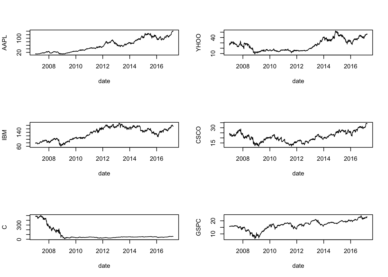
par(mfrow=c(1,1)) #Set the plot figure back to a single plot4.1.5 Convert the data into returns
These are continuously compounded returns, or log returns.
n = length(stock_table[,1])
rets = stock_table[,2:(length(tickers)+1)]
for (j in 1:length(tickers)) {
  rets[2:n,j] = diff(log(rets[,j]))
}
rets$dt = stock_table$dt
rets = rets[2:n,]   #lose the first row when converting to returns
print(head(rets))
## AAPL.Adjusted YHOO.Adjusted IBM.Adjusted CSCO.Adjusted C.Adjusted
## 2 0.021952895 0.047282882 0.010635146 0.0259847487 -0.003444886
## 3 -0.007146715 0.032609594 -0.009094219 0.0003512839 -0.005280834
## 4 0.004926208 0.006467863 0.015077746 0.0056042360 0.005099241
## 5 0.079799692 -0.012252406 0.011760684 -0.0056042360 -0.008757558
## 6 0.046745798 0.039806285 -0.011861824 0.0073491742 -0.008095767
## 7 -0.012448257 0.017271586 -0.002429871 0.0003486308 0.000738734
## GSPC.Adjusted dt
## 2 -0.0003760369 2007-01-04
## 3 0.0000000000 2007-01-05
## 4 0.0093082361 2007-01-08
## 5 -0.0127373254 2007-01-09
## 6 0.0000000000 2007-01-10
## 7 0.0053269494 2007-01-11class(rets)## [1] "data.frame"4.1.6 Descriptive statistics
The data.frame of returns can be used to present the descriptive statistics of returns.
summary(rets)## AAPL.Adjusted YHOO.Adjusted IBM.Adjusted
## Min. :-0.197470 Min. :-0.2340251 Min. :-0.0864191
## 1st Qu.:-0.008318 1st Qu.:-0.0107879 1st Qu.:-0.0064540
## Median : 0.001008 Median : 0.0003064 Median : 0.0004224
## Mean : 0.000999 Mean : 0.0002333 Mean : 0.0003158
## 3rd Qu.: 0.011628 3rd Qu.: 0.0115493 3rd Qu.: 0.0076022
## Max. : 0.130194 Max. : 0.3918166 Max. : 0.1089889
## CSCO.Adjusted C.Adjusted GSPC.Adjusted
## Min. :-0.1768648 Min. :-0.4946962 Min. :-0.1542612
## 1st Qu.:-0.0076399 1st Qu.:-0.0119556 1st Qu.:-0.0040400
## Median : 0.0003616 Median :-0.0000931 Median : 0.0000000
## Mean : 0.0001430 Mean :-0.0008315 Mean : 0.0001502
## 3rd Qu.: 0.0089725 3rd Qu.: 0.0115179 3rd Qu.: 0.0048274
## Max. : 0.1479930 Max. : 0.4563162 Max. : 0.1967094
## dt
## Length:2566
## Class :character
## Mode :character
##
##
## 4.2 Correlation matrix
Now we compute the correlation matrix of returns.
cor(rets[,1:length(tickers)])## AAPL.Adjusted YHOO.Adjusted IBM.Adjusted CSCO.Adjusted
## AAPL.Adjusted 1.0000000 0.3548475 0.4754687 0.4860619
## YHOO.Adjusted 0.3548475 1.0000000 0.3832693 0.4133302
## IBM.Adjusted 0.4754687 0.3832693 1.0000000 0.5710565
## CSCO.Adjusted 0.4860619 0.4133302 0.5710565 1.0000000
## C.Adjusted 0.3731001 0.3377278 0.4329949 0.4633700
## GSPC.Adjusted 0.2220585 0.1667948 0.1996484 0.2277044
## C.Adjusted GSPC.Adjusted
## AAPL.Adjusted 0.3731001 0.2220585
## YHOO.Adjusted 0.3377278 0.1667948
## IBM.Adjusted 0.4329949 0.1996484
## CSCO.Adjusted 0.4633700 0.2277044
## C.Adjusted 1.0000000 0.3303486
## GSPC.Adjusted 0.3303486 1.00000004.2.1 Correlogram
Show the correlogram for the six return series. This is a useful way to visualize the relationship between all variables in the data set.
library(corrgram)
corrgram(rets[,1:length(tickers)], order=TRUE, lower.panel=panel.ellipse,
upper.panel=panel.pts, text.panel=panel.txt) 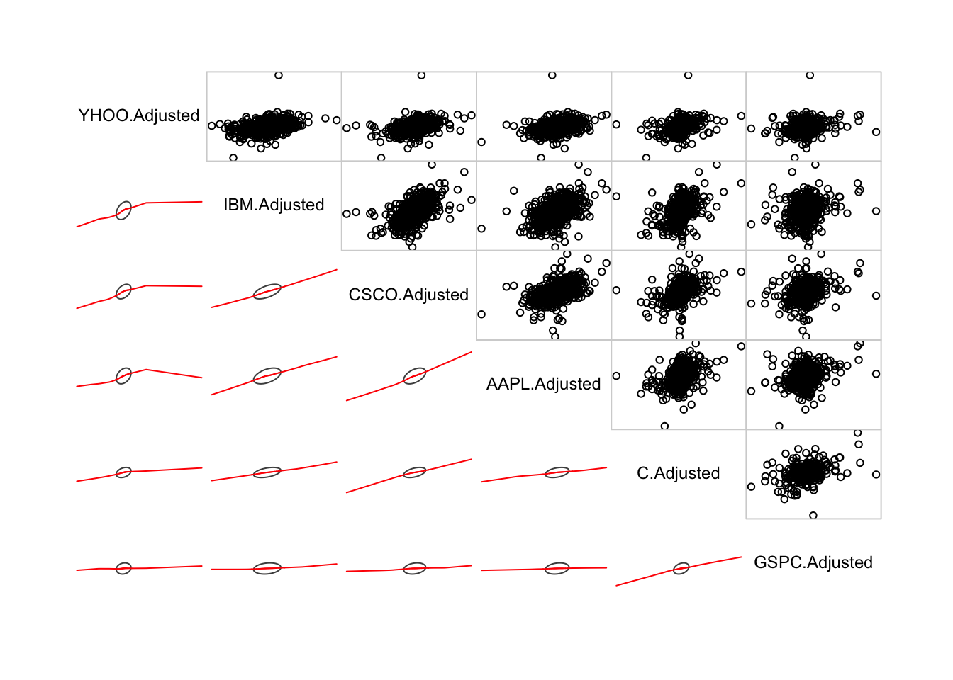
4.2.2 Market regression
To see the relation between the stocks and the index, run a regression of each of the five stocks on the index returns.
betas = NULL
for (j in 1:(length(tickers)-1)) {
  res = lm(rets[,j]~rets[,6])
  betas[j] = res$coefficients[2]
}
print(betas)
## [1] 0.2921709 0.2602061 0.1790612 0.2746572 0.8101568The \(\beta\)s indicate the level of systematic risk for each stock. We notice that all the betas are positive, and highly significant. But they are not close to unity, in fact all are lower. This is evidence of misspecification that may arise from the fact that the stocks are in the tech sector and better explanatory power would come from an index that was more relevant to the technology sector.
4.2.3 Return versus systematic risk
In order to assess whether in the cross-section, there is a relation between average returns and the systematic risk or \(\beta\) of a stock, run a regression of the five average returns on the five betas from the regression.
betas = matrix(betas)
avgrets = colMeans(rets[,1:(length(tickers)-1)])
res = lm(avgrets~betas)
print(summary(res))
##
## Call:
## lm(formula = avgrets ~ betas)
##
## Residuals:
## AAPL.Adjusted YHOO.Adjusted IBM.Adjusted CSCO.Adjusted C.Adjusted
## 6.785e-04 -1.540e-04 -2.411e-04 -2.141e-04 -6.938e-05
##
## Coefficients:
## Estimate Std. Error t value Pr(>|t|)
## (Intercept) 0.0009311 0.0003754 2.480 0.0892 .
## betas -0.0020901 0.0008766 -2.384 0.0972 .
## ---
## Signif. codes: 0 '***' 0.001 '**' 0.01 '*' 0.05 '.' 0.1 ' ' 1
##
## Residual standard error: 0.0004445 on 3 degrees of freedom
## Multiple R-squared: 0.6546, Adjusted R-squared: 0.5394
## F-statistic: 5.685 on 1 and 3 DF, p-value: 0.09724plot(betas,avgrets)
abline(res,col="red")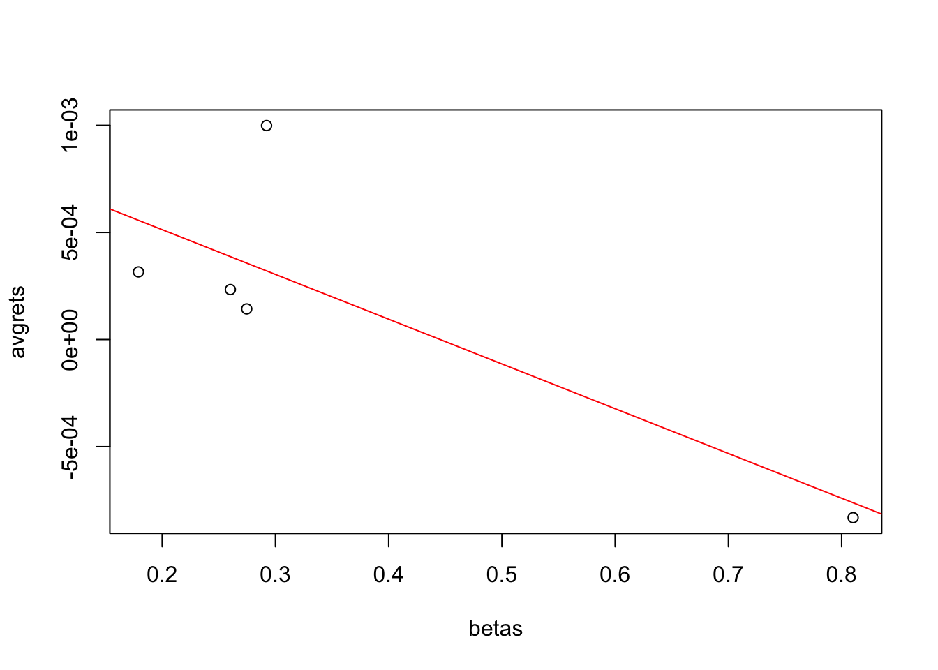
We see indeed, that there is an unexpected negative relation between \(\beta\) and the return levels. This may be on account of the particular small sample we used for illustration here, however, we note that the CAPM (Capital Asset Pricing Model) dictate that we see a positive relation between stock returns and a firm’s systematic risk level.
4.3 Using the merge function
Data frames a very much like spreadsheets or tables, but they are also a lot like databases. Some sort of happy medium. If you want to join two dataframes, it is the same a joining two databases. For this R has the merge function. It is best illustrated with an example.
4.3.1 Extracting online corporate data
Suppose we have a list of ticker symbols and we want to generate a dataframe with more details on these tickers, especially their sector and the full name of the company. Let’s look at the input list of tickers. Suppose I have them in a file called tickers.csv where the delimiter is the colon sign. We read this in as follows.
tickers = read.table("DSTMAA_data/tickers.csv",header=FALSE,sep=":")The line of code reads in the file and this gives us two columns of data. We can look at the top of the file (first 6 rows).
head(tickers)## V1 V2
## 1 NasdaqGS ACOR
## 2 NasdaqGS AKAM
## 3 NYSE ARE
## 4 NasdaqGS AMZN
## 5 NasdaqGS AAPL
## 6 NasdaqGS AREXNote that the ticker symbols relate to stocks from different exchanges, in this case Nasdaq and NYSE. The file may also contain AMEX listed stocks.
The second line of code below counts the number of input tickers, and the third line of code renames the columns of the dataframe. We need to call the column of ticker symbols as ``Symbol’’ because we will see that the dataframe with which we will merge this one also has a column with the same name. This column becomes the index on which the two dataframes are matched and joined.
n = dim(tickers)[1]
print(n)
## [1] 98names(tickers) = c("Exchange","Symbol")
head(tickers)## Exchange Symbol
## 1 NasdaqGS ACOR
## 2 NasdaqGS AKAM
## 3 NYSE ARE
## 4 NasdaqGS AMZN
## 5 NasdaqGS AAPL
## 6 NasdaqGS AREX4.3.2 Get all stock symbols from exchanges
Next, we read in lists of all stocks on Nasdaq, NYSE, and AMEX as follows:
library(quantmod)
nasdaq_names = stockSymbols(exchange="NASDAQ")
## Fetching NASDAQ symbols...nyse_names = stockSymbols(exchange="NYSE")## Fetching NYSE symbols...amex_names = stockSymbols(exchange="AMEX")## Fetching AMEX symbols...We can look at the top of the Nasdaq file.
head(nasdaq_names)## Symbol Name LastSale MarketCap IPOyear
## 1 AAAP Advanced Accelerator Applications S.A. 39.68 $1.72B 2015
## 2 AAL American Airlines Group, Inc. 41.42 $20.88B NA
## 3 AAME Atlantic American Corporation 3.90 $79.62M NA
## 4 AAOI Applied Optoelectronics, Inc. 51.51 $962.1M 2013
## 5 AAON AAON, Inc. 36.40 $1.92B NA
## 6 AAPC Atlantic Alliance Partnership Corp. 9.80 $36.13M 2015
## Sector Industry Exchange
## 1 Health Care Major Pharmaceuticals NASDAQ
## 2 Transportation Air Freight/Delivery Services NASDAQ
## 3 Finance Life Insurance NASDAQ
## 4 Technology Semiconductors NASDAQ
## 5 Capital Goods Industrial Machinery/Components NASDAQ
## 6 Consumer Services Services-Misc. Amusement & Recreation NASDAQNext we merge all three dataframes for each of the exchanges into one data frame.
co_names = rbind(nyse_names,nasdaq_names,amex_names)To see how many rows are there in this merged file, we check dimensions.
dim(co_names)## [1] 6692 8Finally, use the merge function to combine the ticker symbols file with the exchanges data to extend the tickers file to include the information from the exchanges file.
result = merge(tickers,co_names,by="Symbol")
head(result)
## Symbol Exchange.x Name LastSale
## 1 AAPL NasdaqGS Apple Inc. 140.94
## 2 ACOR NasdaqGS Acorda Therapeutics, Inc. 25.35
## 3 AKAM NasdaqGS Akamai Technologies, Inc. 63.67
## 4 AMZN NasdaqGS Amazon.com, Inc. 847.38
## 5 ARE NYSE Alexandria Real Estate Equities, Inc. 112.09
## 6 AREX NasdaqGS Approach Resources Inc. 2.28
## MarketCap IPOyear Sector
## 1 $739.45B 1980 Technology
## 2 $1.18B 2006 Health Care
## 3 $11.03B 1999 Miscellaneous
## 4 $404.34B 1997 Consumer Services
## 5 $10.73B NA Consumer Services
## 6 $184.46M 2007 Energy
## Industry Exchange.y
## 1 Computer Manufacturing NASDAQ
## 2 Biotechnology: Biological Products (No Diagnostic Substances) NASDAQ
## 3 Business Services NASDAQ
## 4 Catalog/Specialty Distribution NASDAQ
## 5 Real Estate Investment Trusts NYSE
## 6 Oil & Gas Production NASDAQAn alternate package to download stock tickers en masse is BatchGetSymbols.
4.4 Using the DT package
The Data Table package is a very good way to examine tabular data through an R-driven user interface.
library(DT)
datatable(co_names, options = list(pageLength = 25))
4.5 Web scraping
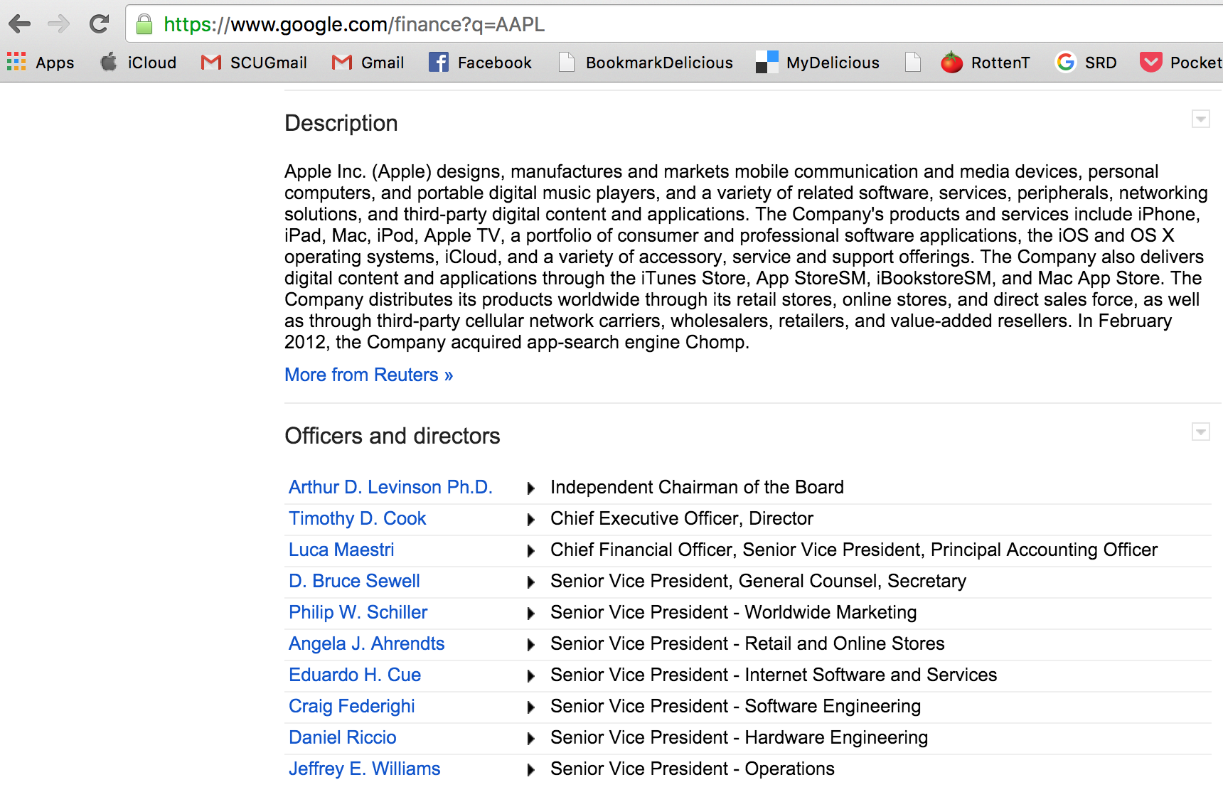
Now suppose we want to find the CEOs of these 98 companies. There is no one file with compay CEO listings freely available for download. However, sites like Google Finance have a page for each stock and mention the CEOs name on the page. By writing R code to scrape the data off these pages one by one, we can extract these CEO names and augment the tickers dataframe. The code for this is simple in R.
library(stringr)

#READ IN THE LIST OF TICKERS
tickers = read.table("DSTMAA_data/tickers.csv",header=FALSE,sep=":")
n = dim(tickers)[1]
names(tickers) = c("Exchange","Symbol")
tickers$ceo = NA

#PULL CEO NAMES FROM GOOGLE FINANCE (take random 10 firms)
for (j in sample(1:n,10)) {
  url = paste("https://www.google.com/finance?q=",tickers[j,2],sep="")
  text = readLines(url)
  idx = grep("Chief Executive",text)
  if (length(idx)>0) {
    tickers[j,3] = str_split(text[idx-2],">")[[1]][2]
  }
  else {
    tickers[j,3] = NA
  }
  print(tickers[j,])
}
## Exchange Symbol ceo
## 19 NasdaqGS FORR George F. Colony
## Exchange Symbol ceo
## 23 NYSE GDOT Steven W. Streit
## Exchange Symbol ceo
## 6 NasdaqGS AREX J. Ross Craft P.E.
## Exchange Symbol ceo
## 33 NYSE IPI Robert P Jornayvaz III
## Exchange Symbol ceo
## 96 NasdaqGS WERN Derek J. Leathers
## Exchange Symbol ceo
## 93 NasdaqGS VSAT Mark D. Dankberg
## Exchange Symbol ceo
## 94 NasdaqGS VRTU Krishan A. Canekeratne
## Exchange Symbol ceo
## 1 NasdaqGS ACOR Ron Cohen M.D.
## Exchange Symbol ceo
## 4 NasdaqGS AMZN Jeffrey P. Bezos
## Exchange Symbol ceo
## 90 NasdaqGS VASC <NA>#WRITE CEO_NAMES TO CSV
write.table(tickers,file="DSTMAA_data/ceo_names.csv",
row.names=FALSE,sep=",")The code uses the stringr package so that string handling is simplified. After extracting the page, we search for the line in which the words ``Chief Executive’’ show up, and we note that the name of the CEO appears two lines before in the html page. A sample web page for Apple Inc is shown here:
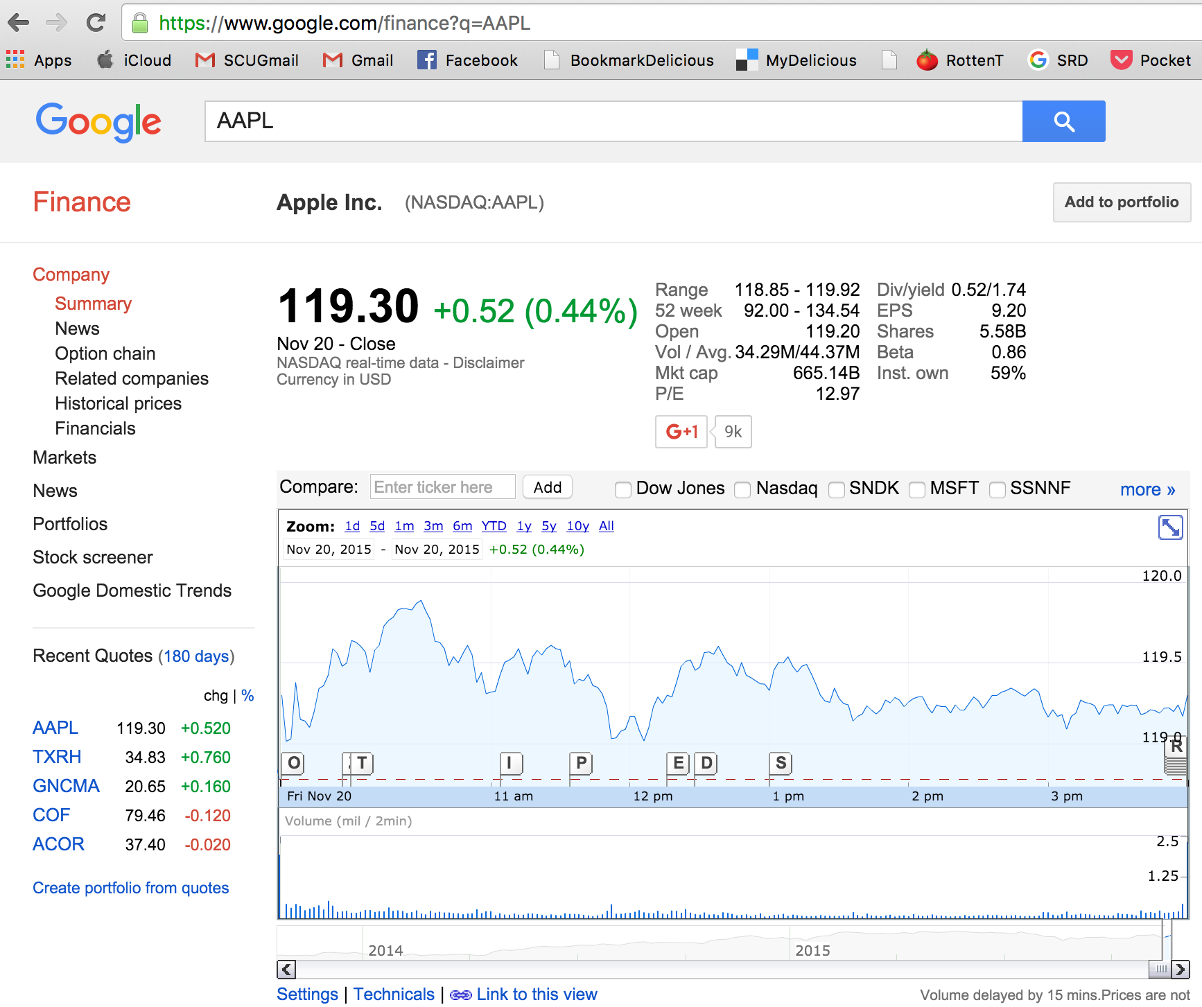
The final dataframe with CEO names is shown here (the top 6 lines):
head(tickers)## Exchange Symbol ceo
## 1 NasdaqGS ACOR Ron Cohen M.D.
## 2 NasdaqGS AKAM <NA>
## 3 NYSE ARE <NA>
## 4 NasdaqGS AMZN Jeffrey P. Bezos
## 5 NasdaqGS AAPL <NA>
## 6 NasdaqGS AREX J. Ross Craft P.E.4.6 Using the apply class of functions
Sometimes we need to apply a function to many cases, and these case parameters may be supplied in a vector, matrix, or list. This is analogous to looping through a set of values to repeat evaluations of a function using different sets of parameters. We illustrate here by computing the mean returns of all stocks in our sample using the apply function. The first argument of the function is the data.frame to which it is being applied, the second argument is either 1 (by rows) or 2 (by columns). The third argument is the function being evaluated.
tickers = c("AAPL","YHOO","IBM","CSCO","C","GSPC")
apply(rets[,1:(length(tickers)-1)],2,mean)
## AAPL.Adjusted YHOO.Adjusted IBM.Adjusted CSCO.Adjusted C.Adjusted
## 0.0009989766 0.0002332882 0.0003158174 0.0001430246 -0.0008315260We see that the function returns the column means of the data set. The variants of the function pertain to what the loop is being applied to. The lapply is a function applied to a list, and sapply is for matrices and vectors. Likewise, mapply uses multiple arguments.
To cross check, we can simply use the colMeans function:
colMeans(rets[,1:(length(tickers)-1)])## AAPL.Adjusted YHOO.Adjusted IBM.Adjusted CSCO.Adjusted C.Adjusted
## 0.0009989766 0.0002332882 0.0003158174 0.0001430246 -0.0008315260As we see, this result is verified.
4.7 Getting interest rate data from FRED
In finance, data on interest rates is widely used. An authoritative source of data on interest rates is FRED (Federal Reserve Economic Data), maintained by the St. Louis Federal Reserve Bank, and is warehoused at the following web site: https://research.stlouisfed.org/fred2/. Let’s assume that we want to download the data using R from FRED directly. To do this we need to write some custom code. There used to be a package for this but since the web site changed, it has been updated but does not work properly. Still, see that it is easy to roll your own code quite easily in R.
#FUNCTION TO READ IN CSV FILES FROM FRED
#Enter SeriesID as a text string
readFRED = function(SeriesID) {
  url = paste("https://research.stlouisfed.org/fred2/series/",
          SeriesID, "/downloaddata/",SeriesID,".csv",sep="")
  data = readLines(url)
  n = length(data)
  data = data[2:n]
  n = length(data)
  df = matrix(0,n,2)   #top line is header
  for (j in 1:n) {
    tmp = strsplit(data[j],",")
    df[j,1] = tmp[[1]][1]
    df[j,2] = tmp[[1]][2]
  }
  rate = as.numeric(df[,2])
  idx = which(rate>0)
  idx = setdiff(seq(1,n),idx)
  rate[idx] = -99
  date = df[,1]
  df = data.frame(date,rate)
  names(df)[2] = SeriesID
  result = df
}
4.7.1 Using the custom function
Now, we provide a list of economic time series and download data accordingly using the function above. Note that we also join these individual series using the data as index. We download constant maturity interest rates (yields) starting from a maturity of one month (DGS1MO) to a maturity of thirty years (DGS30).
#EXTRACT TERM STRUCTURE DATA FOR ALL RATES FROM 1 MO to 30 YRS FROM FRED
id_list = c("DGS1MO","DGS3MO","DGS6MO","DGS1","DGS2","DGS3",
            "DGS5","DGS7","DGS10","DGS20","DGS30")
k = 0
for (id in id_list) {
  out = readFRED(id)
  if (k>0) { rates = merge(rates,out,"date",all=TRUE) }
  else { rates = out }
  k = k + 1
}

head(rates)
## date DGS1MO DGS3MO DGS6MO DGS1 DGS2 DGS3 DGS5 DGS7 DGS10 DGS20
## 1 2001-07-31 3.67 3.54 3.47 3.53 3.79 4.06 4.57 4.86 5.07 5.61
## 2 2001-08-01 3.65 3.53 3.47 3.56 3.83 4.09 4.62 4.90 5.11 5.63
## 3 2001-08-02 3.65 3.53 3.46 3.57 3.89 4.17 4.69 4.97 5.17 5.68
## 4 2001-08-03 3.63 3.52 3.47 3.57 3.91 4.22 4.72 4.99 5.20 5.70
## 5 2001-08-06 3.62 3.52 3.47 3.56 3.88 4.17 4.71 4.99 5.19 5.70
## 6 2001-08-07 3.63 3.52 3.47 3.56 3.90 4.19 4.72 5.00 5.20 5.71
## DGS30
## 1 5.51
## 2 5.53
## 3 5.57
## 4 5.59
## 5 5.59
## 6 5.604.7.2 Organize the data by date
Having done this, we now have a data.frame called rates containing all the time series we are interested in. We now convert the dates into numeric strings and sort the data.frame by date.
#CONVERT ALL DATES TO NUMERIC AND SORT BY DATE
dates = rates[,1]
library(stringr)
dates = as.numeric(str_replace_all(dates,"-",""))
res = sort(dates,index.return=TRUE)
for (j in 1:dim(rates)[2]) {
  rates[,j] = rates[res$ix,j]
}

head(rates)
## date DGS1MO DGS3MO DGS6MO DGS1 DGS2 DGS3 DGS5 DGS7 DGS10 DGS20
## 1 1962-01-02 NA NA NA 3.22 NA 3.70 3.88 NA 4.06 NA
## 2 1962-01-03 NA NA NA 3.24 NA 3.70 3.87 NA 4.03 NA
## 3 1962-01-04 NA NA NA 3.24 NA 3.69 3.86 NA 3.99 NA
## 4 1962-01-05 NA NA NA 3.26 NA 3.71 3.89 NA 4.02 NA
## 5 1962-01-08 NA NA NA 3.31 NA 3.71 3.91 NA 4.03 NA
## 6 1962-01-09 NA NA NA 3.32 NA 3.74 3.93 NA 4.05 NA
## DGS30
## 1 NA
## 2 NA
## 3 NA
## 4 NA
## 5 NA
## 6 NA4.7.3 Handling missing values
Note that there are missing values, denoted by NA. Also there are rows with “-99” values and we can clean those out too but they represent periods when there was no yield available of that maturity, so we leave this in.
#REMOVE THE NA ROWS
idx = which(rowSums(is.na(rates))==0)
rates2 = rates[idx,]
print(head(rates2))
## date DGS1MO DGS3MO DGS6MO DGS1 DGS2 DGS3 DGS5 DGS7 DGS10 DGS20
## 10326 2001-07-31 3.67 3.54 3.47 3.53 3.79 4.06 4.57 4.86 5.07 5.61
## 10327 2001-08-01 3.65 3.53 3.47 3.56 3.83 4.09 4.62 4.90 5.11 5.63
## 10328 2001-08-02 3.65 3.53 3.46 3.57 3.89 4.17 4.69 4.97 5.17 5.68
## 10329 2001-08-03 3.63 3.52 3.47 3.57 3.91 4.22 4.72 4.99 5.20 5.70
## 10330 2001-08-06 3.62 3.52 3.47 3.56 3.88 4.17 4.71 4.99 5.19 5.70
## 10331 2001-08-07 3.63 3.52 3.47 3.56 3.90 4.19 4.72 5.00 5.20 5.71
## DGS30
## 10326 5.51
## 10327 5.53
## 10328 5.57
## 10329 5.59
## 10330 5.59
## 10331 5.604.8 Cross-Sectional Data (an example)
- A great resource for data sets in corporate finance is on Aswath Damodaran’s web site, see: http://people.stern.nyu.edu/adamodar/New_Home_Page/data.html
- Financial statement data sets are available at: http://www.sec.gov/dera/data/financial-statement-data-sets.html
- And another comprehensive data source: http://fisher.osu.edu/fin/fdf/osudata.htm
- Open government data: https://www.data.gov/finance/
Let’s read in the list of failed banks: http://www.fdic.gov/bank/individual/failed/banklist.csv
#download.file(url="http://www.fdic.gov/bank/individual/
#failed/banklist.csv",destfile="failed_banks.csv")
(This does not work, and has been an issue for a while.)
4.8.1 Access file from the web using the readLines function
You can also read in the data using readLines but then further work is required to clean it up, but it works well in downloading the data.
url = "https://www.fdic.gov/bank/individual/failed/banklist.csv"
data = readLines(url)
head(data)
## [1] "Bank Name,City,ST,CERT,Acquiring Institution,Closing Date,Updated Date"
## [2] "Proficio Bank,Cottonwood Heights,UT,35495,Cache Valley Bank,3-Mar-17,14-Mar-17"
## [3] "Seaway Bank and Trust Company,Chicago,IL,19328,State Bank of Texas,27-Jan-17,17-Feb-17"
## [4] "Harvest Community Bank,Pennsville,NJ,34951,First-Citizens Bank & Trust Company,13-Jan-17,17-Feb-17"
## [5] "Allied Bank,Mulberry,AR,91,Today's Bank,23-Sep-16,17-Nov-16"
## [6] "The Woodbury Banking Company,Woodbury,GA,11297,United Bank,19-Aug-16,17-Nov-16"4.8.1.1 Or, read the file from disk
It may be simpler to just download the data and read it in from the csv file:
data = read.csv("DSTMAA_data/banklist.csv",header=TRUE)
print(names(data))
## [1] "Bank.Name" "City" "ST"
## [4] "CERT" "Acquiring.Institution" "Closing.Date"
## [7] "Updated.Date"This gives a data.frame which is easy to work with. We will illustrate some interesting ways in which to manipulate this data.
4.8.2 Failed banks by State
Suppose we want to get subtotals of how many banks failed by state. First add a column of ones to the data.frame.
print(head(data))## Bank.Name City ST CERT
## 1 Banks of Wisconsin d/b/a Bank of Kenosha Kenosha WI 35386
## 2 Central Arizona Bank Scottsdale AZ 34527
## 3 Sunrise Bank Valdosta GA 58185
## 4 Pisgah Community Bank Asheville NC 58701
## 5 Douglas County Bank Douglasville GA 21649
## 6 Parkway Bank Lenoir NC 57158
## Acquiring.Institution Closing.Date Updated.Date
## 1 North Shore Bank, FSB 31-May-13 31-May-13
## 2 Western State Bank 14-May-13 20-May-13
## 3 Synovus Bank 10-May-13 21-May-13
## 4 Capital Bank, N.A. 10-May-13 14-May-13
## 5 Hamilton State Bank 26-Apr-13 16-May-13
## 6 CertusBank, National Association 26-Apr-13 17-May-13data$count = 1
print(head(data))## Bank.Name City ST CERT
## 1 Banks of Wisconsin d/b/a Bank of Kenosha Kenosha WI 35386
## 2 Central Arizona Bank Scottsdale AZ 34527
## 3 Sunrise Bank Valdosta GA 58185
## 4 Pisgah Community Bank Asheville NC 58701
## 5 Douglas County Bank Douglasville GA 21649
## 6 Parkway Bank Lenoir NC 57158
## Acquiring.Institution Closing.Date Updated.Date count
## 1 North Shore Bank, FSB 31-May-13 31-May-13 1
## 2 Western State Bank 14-May-13 20-May-13 1
## 3 Synovus Bank 10-May-13 21-May-13 1
## 4 Capital Bank, N.A. 10-May-13 14-May-13 1
## 5 Hamilton State Bank 26-Apr-13 16-May-13 1
## 6 CertusBank, National Association 26-Apr-13 17-May-13 14.8.2.1 Check for missing data
It’s good to check that there is no missing data.
any(is.na(data))## [1] FALSE4.8.2.2 Sort by State
Now we sort the data by state to see how many there are.
res = sort(as.matrix(data$ST),index.return=TRUE)
print(head(data[res$ix,]))
## Bank.Name City ST CERT
## 42 Alabama Trust Bank, National Association Sylacauga AL 35224
## 126 Superior Bank Birmingham AL 17750
## 127 Nexity Bank Birmingham AL 19794
## 279 First Lowndes Bank Fort Deposit AL 24957
## 318 New South Federal Savings Bank Irondale AL 32276
## 375 CapitalSouth Bank Birmingham AL 22130
## Acquiring.Institution Closing.Date Updated.Date count
## 42 Southern States Bank 18-May-12 20-May-13 1
## 126 Superior Bank, National Association 15-Apr-11 30-Nov-12 1
## 127 AloStar Bank of Commerce 15-Apr-11 4-Sep-12 1
## 279 First Citizens Bank 19-Mar-10 23-Aug-12 1
## 318 Beal Bank 18-Dec-09 23-Aug-12 1
## 375 IBERIABANK 21-Aug-09 15-Jan-13 1print(head(sort(unique(data$ST))))## [1] AL AR AZ CA CO CT
## 44 Levels: AL AR AZ CA CO CT FL GA HI IA ID IL IN KS KY LA MA MD MI ... WYprint(length(unique(data$ST)))## [1] 444.8.3 Use the aggregate function (for subtotals)
We can directly use the aggregate function to get subtotals by state.
head(aggregate(count ~ ST,data,sum),10)## ST count
## 1 AL 7
## 2 AR 3
## 3 AZ 15
## 4 CA 40
## 5 CO 9
## 6 CT 1
## 7 FL 71
## 8 GA 89
## 9 HI 1
## 10 IA 14.8.3.1 Data by acquiring bank
And another example, subtotal by acquiring bank. Note how we take the subtotals into another data.frame, which is then sorted and returned in order using the index of the sort.
acq = aggregate(count~Acquiring.Institution,data,sum)
idx = sort(as.matrix(acq$count),decreasing=TRUE,index.return=TRUE)$ix
head(acq[idx,],15)
## Acquiring.Institution count
## 158 No Acquirer 30
## 208 State Bank and Trust Company 12
## 9 Ameris Bank 10
## 245 U.S. Bank N.A. 9
## 25 Bank of the Ozarks 7
## 41 Centennial Bank 7
## 61 Community & Southern Bank 7
## 212 Stearns Bank, N.A. 7
## 43 CenterState Bank of Florida, N.A. 6
## 44 Central Bank 6
## 103 First-Citizens Bank & Trust Company 6
## 143 MB Financial Bank, N.A. 6
## 48 CertusBank, National Association 5
## 58 Columbia State Bank 5
## 178 Premier American Bank, N.A. 54.9 Handling dates with lubridate
Suppose we want to take the preceding data.frame of failed banks and aggregate the data by year, or month, etc. In this case, it us useful to use a dates package. Another useful tool developed by Hadley Wickham is the lubridate package.
head(data)## Bank.Name City ST CERT
## 1 Banks of Wisconsin d/b/a Bank of Kenosha Kenosha WI 35386
## 2 Central Arizona Bank Scottsdale AZ 34527
## 3 Sunrise Bank Valdosta GA 58185
## 4 Pisgah Community Bank Asheville NC 58701
## 5 Douglas County Bank Douglasville GA 21649
## 6 Parkway Bank Lenoir NC 57158
## Acquiring.Institution Closing.Date Updated.Date count
## 1 North Shore Bank, FSB 31-May-13 31-May-13 1
## 2 Western State Bank 14-May-13 20-May-13 1
## 3 Synovus Bank 10-May-13 21-May-13 1
## 4 Capital Bank, N.A. 10-May-13 14-May-13 1
## 5 Hamilton State Bank 26-Apr-13 16-May-13 1
## 6 CertusBank, National Association 26-Apr-13 17-May-13 1library(lubridate)##
## Attaching package: 'lubridate'## The following object is masked from 'package:base':
##
## datedata$Cdate = dmy(data$Closing.Date)
data$Cyear = year(data$Cdate)
fd = aggregate(count~Cyear,data,sum)
print(fd)## Cyear count
## 1 2000 2
## 2 2001 4
## 3 2002 11
## 4 2003 3
## 5 2004 4
## 6 2007 3
## 7 2008 25
## 8 2009 140
## 9 2010 157
## 10 2011 92
## 11 2012 51
## 12 2013 14plot(count~Cyear,data=fd,type="l",lwd=3,col="red",xlab="Year")
grid(lwd=3)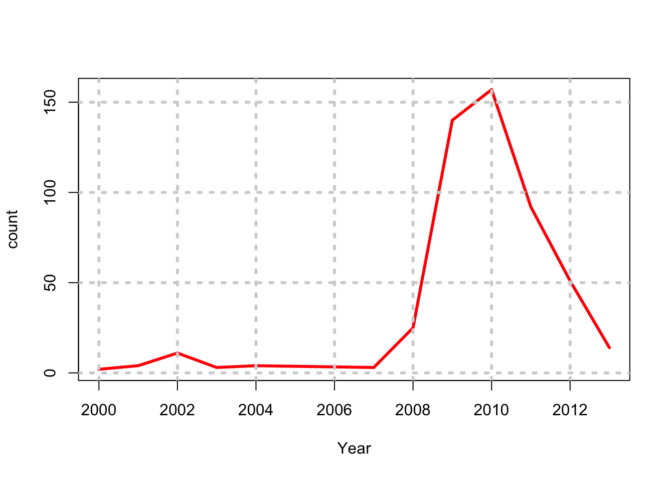
4.9.1 By Month
Let’s do the same thing by month to see if there is seasonality
data$Cmonth = month(data$Cdate)
fd = aggregate(count~Cmonth,data,sum)
print(fd)
## Cmonth count
## 1 1 44
## 2 2 40
## 3 3 38
## 4 4 56
## 5 5 36
## 6 6 31
## 7 7 71
## 8 8 36
## 9 9 35
## 10 10 53
## 11 11 34
## 12 12 32plot(count~Cmonth,data=fd,type="l",lwd=3,col="green"); grid(lwd=3)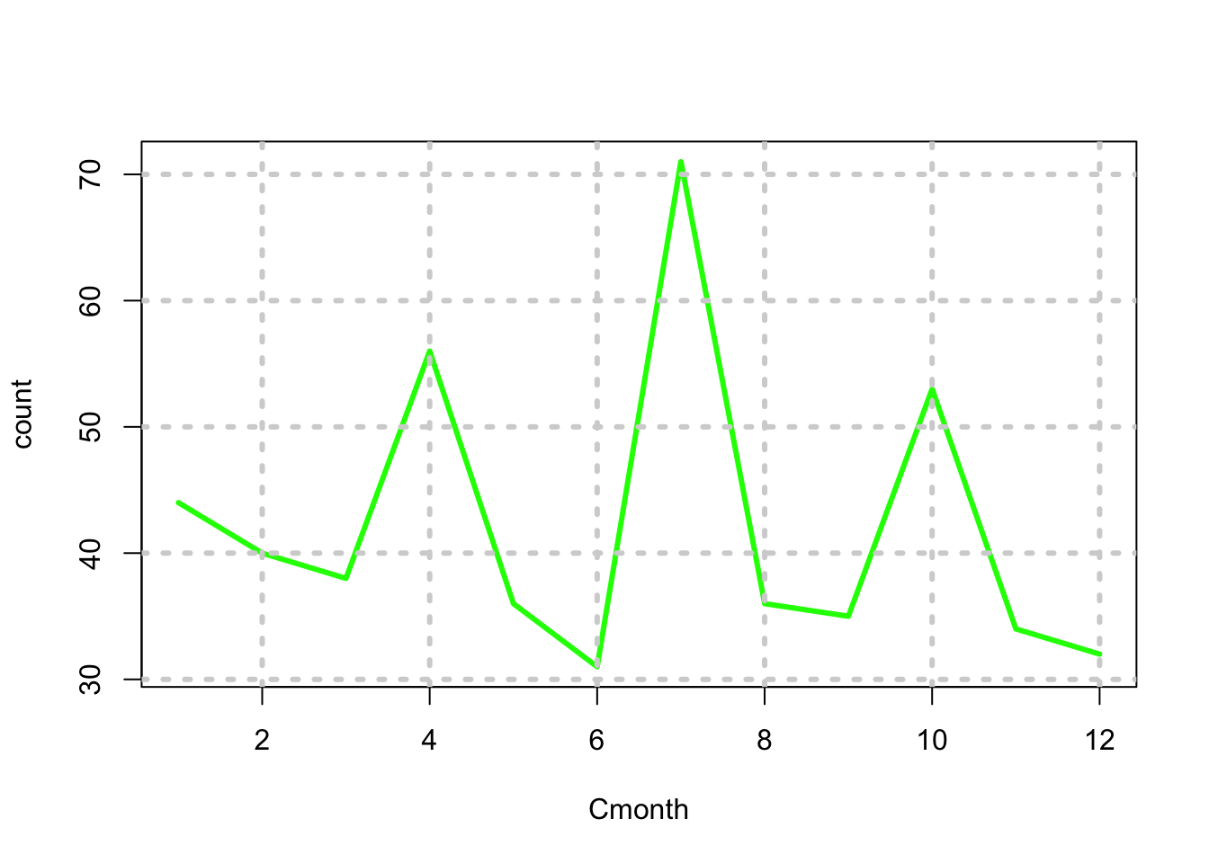
4.9.2 By Day
There does not appear to be any seasonality. What about day?
data$Cday = day(data$Cdate)
fd = aggregate(count~Cday,data,sum)
print(fd)
## Cday count
## 1 1 8
## 2 2 17
## 3 3 3
## 4 4 21
## 5 5 15
## 6 6 12
## 7 7 18
## 8 8 13
## 9 9 9
## 10 10 13
## 11 11 17
## 12 12 10
## 13 13 10
## 14 14 20
## 15 15 20
## 16 16 20
## 17 17 21
## 18 18 20
## 19 19 28
## 20 20 25
## 21 21 17
## 22 22 18
## 23 23 26
## 24 24 17
## 25 25 11
## 26 26 15
## 27 27 16
## 28 28 16
## 29 29 15
## 30 30 28
## 31 31 7plot(count~Cday,data=fd,type="l",lwd=3,col="blue"); grid(lwd=3)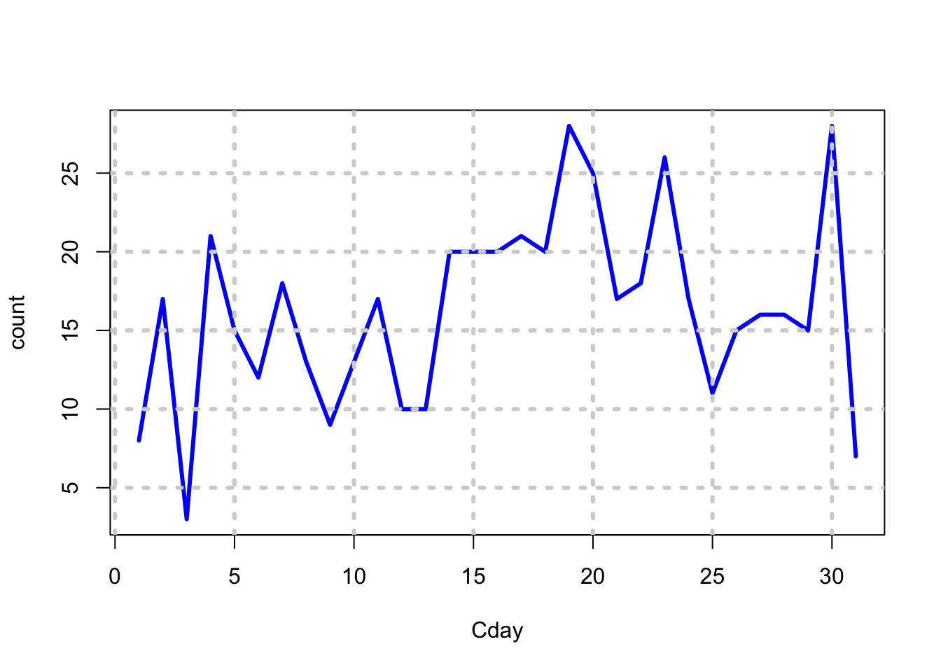
Definitely, counts are lower at the start and end of the month!
4.10 Using the data.table package
This is an incredibly useful package that was written by Matt Dowle. It essentially allows your data.frame to operate as a database. It enables very fast handling of massive quantities of data, and much of this technology is now embedded in the IP of the company called h2o: http://h2o.ai/
The data.table cheat sheet is here: https://s3.amazonaws.com/assets.datacamp.com/img/blog/data+table+cheat+sheet.pdf
4.10.1 California Crime Statistics
We start with some freely downloadable crime data statistics for California. We placed the data in a csv file which is then easy to read in to R.
data = read.csv("DSTMAA_data/CA_Crimes_Data_2004-2013.csv",header=TRUE)It is easy to convert this into a data.table.
library(data.table)##
## Attaching package: 'data.table'## The following objects are masked from 'package:lubridate':
##
## hour, mday, month, quarter, wday, week, yday, year## The following object is masked from 'package:xts':
##
## lastD_T = as.data.table(data)
print(class(D_T)) ## [1] "data.table" "data.frame"Note, it is still a data.frame also. Hence, it inherits its properties from the data.frame class.
4.10.2 Examine the data.table
Let’s see how it works, noting that the syntax is similar to that for data.frames as much as possible. We print only a part of the names list. And do not go through each and everyone.
print(dim(D_T))## [1] 7301 69print(names(D_T))## [1] "Year" "County" "NCICCode"
## [4] "Violent_sum" "Homicide_sum" "ForRape_sum"
## [7] "Robbery_sum" "AggAssault_sum" "Property_sum"
## [10] "Burglary_sum" "VehicleTheft_sum" "LTtotal_sum"
## [13] "ViolentClr_sum" "HomicideClr_sum" "ForRapeClr_sum"
## [16] "RobberyClr_sum" "AggAssaultClr_sum" "PropertyClr_sum"
## [19] "BurglaryClr_sum" "VehicleTheftClr_sum" "LTtotalClr_sum"
## [22] "TotalStructural_sum" "TotalMobile_sum" "TotalOther_sum"
## [25] "GrandTotal_sum" "GrandTotClr_sum" "RAPact_sum"
## [28] "ARAPact_sum" "FROBact_sum" "KROBact_sum"
## [31] "OROBact_sum" "SROBact_sum" "HROBnao_sum"
## [34] "CHROBnao_sum" "GROBnao_sum" "CROBnao_sum"
## [37] "RROBnao_sum" "BROBnao_sum" "MROBnao_sum"
## [40] "FASSact_sum" "KASSact_sum" "OASSact_sum"
## [43] "HASSact_sum" "FEBURact_Sum" "UBURact_sum"
## [46] "RESDBUR_sum" "RNBURnao_sum" "RDBURnao_sum"
## [49] "RUBURnao_sum" "NRESBUR_sum" "NNBURnao_sum"
## [52] "NDBURnao_sum" "NUBURnao_sum" "MVTact_sum"
## [55] "TMVTact_sum" "OMVTact_sum" "PPLARnao_sum"
## [58] "PSLARnao_sum" "SLLARnao_sum" "MVLARnao_sum"
## [61] "MVPLARnao_sum" "BILARnao_sum" "FBLARnao_sum"
## [64] "COMLARnao_sum" "AOLARnao_sum" "LT400nao_sum"
## [67] "LT200400nao_sum" "LT50200nao_sum" "LT50nao_sum"head(D_T)## Year County NCICCode Violent_sum
## 1: 2004 Alameda County Alameda Co. Sheriff's Department 461
## 2: 2004 Alameda County Alameda 342
## 3: 2004 Alameda County Albany 42
## 4: 2004 Alameda County Berkeley 557
## 5: 2004 Alameda County Emeryville 83
## 6: 2004 Alameda County Fremont 454
## Homicide_sum ForRape_sum Robbery_sum AggAssault_sum Property_sum
## 1: 5 29 174 253 3351
## 2: 1 12 89 240 2231
## 3: 1 3 29 9 718
## 4: 4 17 355 181 8611
## 5: 2 4 53 24 1066
## 6: 5 24 165 260 5723
## Burglary_sum VehicleTheft_sum LTtotal_sum ViolentClr_sum
## 1: 731 947 1673 170
## 2: 376 333 1522 244
## 3: 130 142 446 10
## 4: 1382 1128 6101 169
## 5: 94 228 744 15
## 6: 939 881 3903 232
## HomicideClr_sum ForRapeClr_sum RobberyClr_sum AggAssaultClr_sum
## 1: 5 4 43 118
## 2: 1 8 45 190
## 3: 0 1 3 6
## 4: 1 6 72 90
## 5: 1 0 8 6
## 6: 2 18 51 161
## PropertyClr_sum BurglaryClr_sum VehicleTheftClr_sum LTtotalClr_sum
## 1: 275 58 129 88
## 2: 330 65 57 208
## 3: 53 24 2 27
## 4: 484 58 27 399
## 5: 169 14 4 151
## 6: 697 84 135 478
## TotalStructural_sum TotalMobile_sum TotalOther_sum GrandTotal_sum
## 1: 7 23 3 33
## 2: 5 1 9 15
## 3: 3 0 5 8
## 4: 21 21 17 59
## 5: 0 1 0 1
## 6: 8 10 3 21
## GrandTotClr_sum RAPact_sum ARAPact_sum FROBact_sum KROBact_sum
## 1: 4 27 2 53 17
## 2: 5 12 0 18 4
## 3: 0 3 0 9 1
## 4: 15 12 5 126 20
## 5: 0 4 0 13 6
## 6: 5 23 1 64 22
## OROBact_sum SROBact_sum HROBnao_sum CHROBnao_sum GROBnao_sum
## 1: 9 95 81 19 6
## 2: 11 56 49 14 0
## 3: 1 18 21 1 0
## 4: 71 138 201 58 6
## 5: 1 33 33 11 2
## 6: 6 73 89 19 3
## CROBnao_sum RROBnao_sum BROBnao_sum MROBnao_sum FASSact_sum KASSact_sum
## 1: 13 17 13 25 17 35
## 2: 3 9 4 10 8 23
## 3: 1 2 3 1 0 3
## 4: 2 24 22 42 15 16
## 5: 1 1 0 5 4 0
## 6: 28 2 12 12 19 56
## OASSact_sum HASSact_sum FEBURact_Sum UBURact_sum RESDBUR_sum
## 1: 132 69 436 295 538
## 2: 86 123 183 193 213
## 3: 4 2 61 69 73
## 4: 73 77 748 634 962
## 5: 9 11 61 33 36
## 6: 120 65 698 241 593
## RNBURnao_sum RDBURnao_sum RUBURnao_sum NRESBUR_sum NNBURnao_sum
## 1: 131 252 155 193 76
## 2: 40 67 106 163 31
## 3: 11 60 2 57 25
## 4: 225 418 319 420 171
## 5: 8 25 3 58 40
## 6: 106 313 174 346 76
## NDBURnao_sum NUBURnao_sum MVTact_sum TMVTact_sum OMVTact_sum
## 1: 33 84 879 2 66
## 2: 18 114 250 59 24
## 3: 31 1 116 21 5
## 4: 112 137 849 169 110
## 5: 14 4 182 33 13
## 6: 34 236 719 95 67
## PPLARnao_sum PSLARnao_sum SLLARnao_sum MVLARnao_sum MVPLARnao_sum
## 1: 14 14 76 1048 56
## 2: 0 1 176 652 14
## 3: 1 2 27 229 31
## 4: 22 34 376 2373 1097
## 5: 17 2 194 219 122
## 6: 3 26 391 2269 325
## BILARnao_sum FBLARnao_sum COMLARnao_sum AOLARnao_sum LT400nao_sum
## 1: 54 192 5 214 681
## 2: 176 172 8 323 371
## 3: 47 60 1 48 76
## 4: 374 539 7 1279 1257
## 5: 35 44 0 111 254
## 6: 79 266 13 531 1298
## LT200400nao_sum LT50200nao_sum LT50nao_sum
## 1: 301 308 383
## 2: 274 336 541
## 3: 101 120 149
## 4: 1124 1178 2542
## 5: 110 141 239
## 6: 663 738 12044.10.3 Indexing the data.table
A nice feature of the data.table is that it can be indexed, i.e., resorted on the fly by making any column in the database the key. Once that is done, then it becomes easy to compute subtotals, and generate plots from these subtotals as well.
The data table can be used like a database, and you can directly apply summarization functions to it. Essentially, it is governed by a format that is summarized as (\(i\),\(j\),by), i.e., apply some rule to rows \(i\), then to some columns \(j\), and one may also group by some columns. We can see how this works with the following example.
setkey(D_T,Year)

crime = 6
res = D_T[,sum(ForRape_sum),by=Year]
print(res)
## Year V1
## 1: 2004 9598
## 2: 2005 9345
## 3: 2006 9213
## 4: 2007 9047
## 5: 2008 8906
## 6: 2009 8698
## 7: 2010 8325
## 8: 2011 7678
## 9: 2012 7828
## 10: 2013 7459class(res)## [1] "data.table" "data.frame"The data table was operated on for all columns, i.e., all \(i\), and the \(j\) column we are interested in was the “ForRape_sum” which we want to total by Year. This returns a summary of only the Year and the total number of rapes per year. See that the type of output is also of the type data.table, which includes the class data.frame also.
4.10.4 Plotting from the data.table
Next, we plot the results from the data.table in the same way as we would for a data.frame.
plot(res$Year,res$V1,type="b",lwd=3,col="blue",
    xlab="Year",ylab="Forced Rape")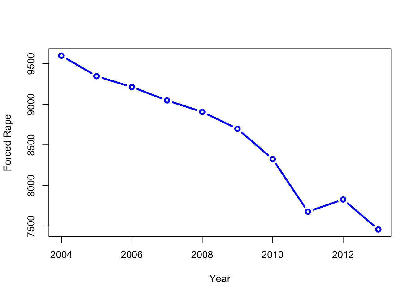
4.10.4.1 By County
Repeat the process looking at crime (Rape) totals by county.
setkey(D_T,County)
res = D_T[,sum(ForRape_sum),by=County]
print(res)
## County V1
## 1: Alameda County 4979
## 2: Alpine County 15
## 3: Amador County 153
## 4: Butte County 930
## 5: Calaveras County 148
## 6: Colusa County 60
## 7: Contra Costa County 1848
## 8: Del Norte County 236
## 9: El Dorado County 351
## 10: Fresno County 1960
## 11: Glenn County 56
## 12: Humboldt County 495
## 13: Imperial County 263
## 14: Inyo County 52
## 15: Kern County 1935
## 16: Kings County 356
## 17: Lake County 262
## 18: Lassen County 96
## 19: Los Angeles County 21483
## 20: Madera County 408
## 21: Marin County 452
## 22: Mariposa County 46
## 23: Mendocino County 328
## 24: Merced County 738
## 25: Modoc County 64
## 26: Mono County 61
## 27: Monterey County 1062
## 28: Napa County 354
## 29: Nevada County 214
## 30: Orange County 4509
## 31: Placer County 611
## 32: Plumas County 115
## 33: Riverside County 4321
## 34: Sacramento County 4084
## 35: San Benito County 151
## 36: San Bernardino County 4900
## 37: San Diego County 7378
## 38: San Francisco County 1498
## 39: San Joaquin County 1612
## 40: San Luis Obispo County 900
## 41: San Mateo County 1381
## 42: Santa Barbara County 1352
## 43: Santa Clara County 3832
## 44: Santa Cruz County 865
## 45: Shasta County 1089
## 46: Sierra County 2
## 47: Siskiyou County 143
## 48: Solano County 1150
## 49: Sonoma County 1558
## 50: Stanislaus County 1348
## 51: Sutter County 274
## 52: Tehama County 165
## 53: Trinity County 28
## 54: Tulare County 1114
## 55: Tuolumne County 160
## 56: Ventura County 1146
## 57: Yolo County 729
## 58: Yuba County 277
## County V1setnames(res,"V1","Rapes")
County_Rapes = as.data.table(res) #This is not really needed
setkey(County_Rapes,Rapes)
print(County_Rapes)## County Rapes
## 1: Sierra County 2
## 2: Alpine County 15
## 3: Trinity County 28
## 4: Mariposa County 46
## 5: Inyo County 52
## 6: Glenn County 56
## 7: Colusa County 60
## 8: Mono County 61
## 9: Modoc County 64
## 10: Lassen County 96
## 11: Plumas County 115
## 12: Siskiyou County 143
## 13: Calaveras County 148
## 14: San Benito County 151
## 15: Amador County 153
## 16: Tuolumne County 160
## 17: Tehama County 165
## 18: Nevada County 214
## 19: Del Norte County 236
## 20: Lake County 262
## 21: Imperial County 263
## 22: Sutter County 274
## 23: Yuba County 277
## 24: Mendocino County 328
## 25: El Dorado County 351
## 26: Napa County 354
## 27: Kings County 356
## 28: Madera County 408
## 29: Marin County 452
## 30: Humboldt County 495
## 31: Placer County 611
## 32: Yolo County 729
## 33: Merced County 738
## 34: Santa Cruz County 865
## 35: San Luis Obispo County 900
## 36: Butte County 930
## 37: Monterey County 1062
## 38: Shasta County 1089
## 39: Tulare County 1114
## 40: Ventura County 1146
## 41: Solano County 1150
## 42: Stanislaus County 1348
## 43: Santa Barbara County 1352
## 44: San Mateo County 1381
## 45: San Francisco County 1498
## 46: Sonoma County 1558
## 47: San Joaquin County 1612
## 48: Contra Costa County 1848
## 49: Kern County 1935
## 50: Fresno County 1960
## 51: Santa Clara County 3832
## 52: Sacramento County 4084
## 53: Riverside County 4321
## 54: Orange County 4509
## 55: San Bernardino County 4900
## 56: Alameda County 4979
## 57: San Diego County 7378
## 58: Los Angeles County 21483
## County Rapes4.10.4.2 Barplot of crime
Now, we can go ahead and plot it using a different kind of plot, a horizontal barplot.
par(las=2)  #makes label horizontal
#par(mar=c(3,4,2,1))  #increase y-axis margins
barplot(County_Rapes$Rapes, names.arg=County_Rapes$County,
horiz=TRUE, cex.names=0.4, col=8)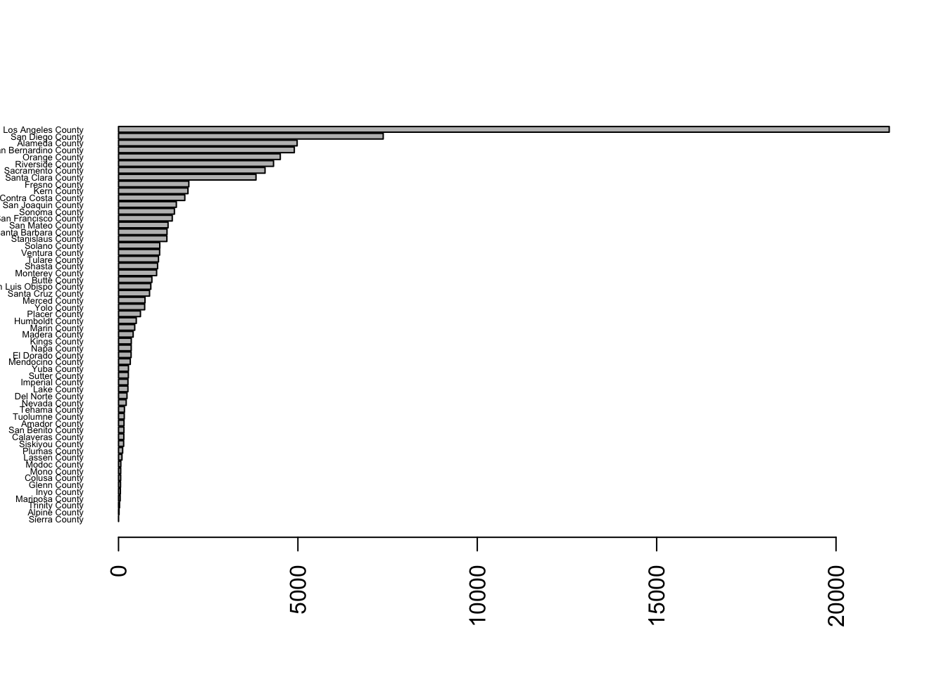
4.11 The plyr package family
This package by Hadley Wickham is useful for applying functions to tables of data, i.e., data.frames. Since we may want to write custom functions, this is a highly useful package. R users often select either the data.table or the plyr class of packages for handling data.frames as databases. The latest incarnation is the dplyr package, which focuses only on data.frames.
require(plyr)## Loading required package: plyr##
## Attaching package: 'plyr'## The following object is masked from 'package:lubridate':
##
## here## The following object is masked from 'package:corrgram':
##
## baseballlibrary(dplyr)## -------------------------------------------------------------------------## data.table + dplyr code now lives in dtplyr.
## Please library(dtplyr)!## -------------------------------------------------------------------------##
## Attaching package: 'dplyr'## The following objects are masked from 'package:plyr':
##
## arrange, count, desc, failwith, id, mutate, rename, summarise,
## summarize## The following objects are masked from 'package:data.table':
##
## between, last## The following objects are masked from 'package:lubridate':
##
## intersect, setdiff, union## The following objects are masked from 'package:xts':
##
## first, last## The following objects are masked from 'package:stats':
##
## filter, lag## The following objects are masked from 'package:base':
##
## intersect, setdiff, setequal, union4.11.1 Filter the data
One of the useful things you can use is the filter function, to subset the rows of the dataset you might want to select for further analysis.
res = filter(trips,Start.Terminal==50,End.Terminal==51)
head(res)
## Trip.ID Duration Start.Date Start.Station
## 1 432024 3954 8/30/2014 14:46 Harry Bridges Plaza (Ferry Building)
## 2 432022 4120 8/30/2014 14:44 Harry Bridges Plaza (Ferry Building)
## 3 431895 1196 8/30/2014 12:04 Harry Bridges Plaza (Ferry Building)
## 4 431891 1249 8/30/2014 12:03 Harry Bridges Plaza (Ferry Building)
## 5 430408 145 8/29/2014 9:08 Harry Bridges Plaza (Ferry Building)
## 6 429148 862 8/28/2014 13:47 Harry Bridges Plaza (Ferry Building)
## Start.Terminal End.Date End.Station End.Terminal Bike..
## 1 50 8/30/2014 15:52 Embarcadero at Folsom 51 306
## 2 50 8/30/2014 15:52 Embarcadero at Folsom 51 659
## 3 50 8/30/2014 12:24 Embarcadero at Folsom 51 556
## 4 50 8/30/2014 12:23 Embarcadero at Folsom 51 621
## 5 50 8/29/2014 9:11 Embarcadero at Folsom 51 400
## 6 50 8/28/2014 14:02 Embarcadero at Folsom 51 589
## Subscriber.Type Zip.Code
## 1 Customer 94952
## 2 Customer 94952
## 3 Customer 11238
## 4 Customer 11238
## 5 Subscriber 94070
## 6 Subscriber 941074.11.2 Sorting using the arrange function
The arrange function is useful for sorting by any number of columns as needed. Here we sort by the start and end stations.
trips_sorted = arrange(trips,Start.Station,End.Station)
head(trips_sorted)
## Trip.ID Duration Start.Date Start.Station Start.Terminal
## 1 426408 120 8/27/2014 7:40 2nd at Folsom 62
## 2 411496 21183 8/16/2014 13:36 2nd at Folsom 62
## 3 396676 3707 8/6/2014 11:38 2nd at Folsom 62
## 4 385761 123 7/29/2014 19:52 2nd at Folsom 62
## 5 364633 6395 7/15/2014 13:39 2nd at Folsom 62
## 6 362776 9433 7/14/2014 13:36 2nd at Folsom 62
## End.Date End.Station End.Terminal Bike.. Subscriber.Type
## 1 8/27/2014 7:42 2nd at Folsom 62 527 Subscriber
## 2 8/16/2014 19:29 2nd at Folsom 62 508 Customer
## 3 8/6/2014 12:40 2nd at Folsom 62 109 Customer
## 4 7/29/2014 19:55 2nd at Folsom 62 421 Subscriber
## 5 7/15/2014 15:26 2nd at Folsom 62 448 Customer
## 6 7/14/2014 16:13 2nd at Folsom 62 454 Customer
## Zip.Code
## 1 94107
## 2 94105
## 3 31200
## 4 94107
## 5 2184
## 6 21844.11.3 Reverse order sort
The sort can also be done in reverse order as follows.
trips_sorted = arrange(trips,desc(Start.Station),End.Station)
head(trips_sorted)
## Trip.ID Duration Start.Date
## 1 416755 285 8/20/2014 11:37
## 2 411270 257 8/16/2014 7:03
## 3 410269 286 8/15/2014 10:34
## 4 405273 382 8/12/2014 14:27
## 5 398372 401 8/7/2014 10:10
## 6 393012 317 8/4/2014 10:59
## Start.Station Start.Terminal
## 1 Yerba Buena Center of the Arts (3rd @ Howard) 68
## 2 Yerba Buena Center of the Arts (3rd @ Howard) 68
## 3 Yerba Buena Center of the Arts (3rd @ Howard) 68
## 4 Yerba Buena Center of the Arts (3rd @ Howard) 68
## 5 Yerba Buena Center of the Arts (3rd @ Howard) 68
## 6 Yerba Buena Center of the Arts (3rd @ Howard) 68
## End.Date End.Station End.Terminal Bike.. Subscriber.Type
## 1 8/20/2014 11:42 2nd at Folsom 62 383 Customer
## 2 8/16/2014 7:07 2nd at Folsom 62 614 Subscriber
## 3 8/15/2014 10:38 2nd at Folsom 62 545 Subscriber
## 4 8/12/2014 14:34 2nd at Folsom 62 344 Customer
## 5 8/7/2014 10:16 2nd at Folsom 62 597 Subscriber
## 6 8/4/2014 11:04 2nd at Folsom 62 367 Subscriber
## Zip.Code
## 1 95060
## 2 94107
## 3 94127
## 4 94110
## 5 94127
## 6 941274.11.4 Descriptive statistics
Data.table also offers a fantastic way to do descriptive statistics! First, group the data by start point, and then produce statistics by this group, choosing to count the number of trips starting from each station and the average duration of each trip.
byStartStation = group_by(trips,Start.Station)
res = summarise(byStartStation, count=n(), time=mean(Duration)/60)
print(res)
## # A tibble: 70 x 3
## Start.Station count time
## <fctr> <int> <dbl>
## 1 2nd at Folsom 4165 9.32088
## 2 2nd at South Park 4569 11.60195
## 3 2nd at Townsend 6824 15.14786
## 4 5th at Howard 3183 14.23254
## 5 Adobe on Almaden 360 10.06120
## 6 Arena Green / SAP Center 510 43.82833
## 7 Beale at Market 4293 15.74702
## 8 Broadway at Main 22 54.82121
## 9 Broadway St at Battery St 2433 15.31862
## 10 California Ave Caltrain Station 329 51.30709
## # ... with 60 more rows4.11.5 Other functions in dplyr
Try also the select(), extract(), mutate(), summarise(), sample_n(), sample_frac() functions.
The group_by() function is particularly useful as we have seen.
4.12 Application to IPO Data
Let’s revisit all the stock exchange data from before, where we download the table of firms listed on the NYSE, NASDAQ, and AMEX using the quantmod package.
library(quantmod)
nasdaq_names = stockSymbols(exchange = "NASDAQ")
## Fetching NASDAQ symbols...nyse_names = stockSymbols(exchange = "NYSE")## Fetching NYSE symbols...amex_names = stockSymbols(exchange = "AMEX")## Fetching AMEX symbols...tickers = rbind(nasdaq_names,nyse_names,amex_names)
tickers$Count = 1
print(dim(tickers))## [1] 6692 9We then clean off the rows with incomplete data, using the very useful complete.cases function.
idx = complete.cases(tickers)
df = tickers[idx,]
print(nrow(df))
## [1] 2198We create a table of the frequency of IPOs by year to see hot and cold IPO markets. 1. First, remove all rows with missing IPO data. 2. Plot IPO Activity with a bar plot. We make sure to label the axes properly. 3. Plot IPO Activity using the rbokeh package to make a pretty line plot. See: https://hafen.github.io/rbokeh/
library(dplyr)
library(magrittr)

idx = which(!is.na(tickers$IPOyear))
df = tickers[idx,]
res = df %>% group_by(IPOyear) %>% summarise(numIPO = sum(Count))
print(res)
## # A tibble: 40 x 2
## IPOyear numIPO
## <int> <dbl>
## 1 1972 4
## 2 1973 1
## 3 1980 2
## 4 1981 6
## 5 1982 4
## 6 1983 13
## 7 1984 6
## 8 1985 4
## 9 1986 38
## 10 1987 28
## # ... with 30 more rowsbarplot(res$numIPO,names.arg = res$IPOyear)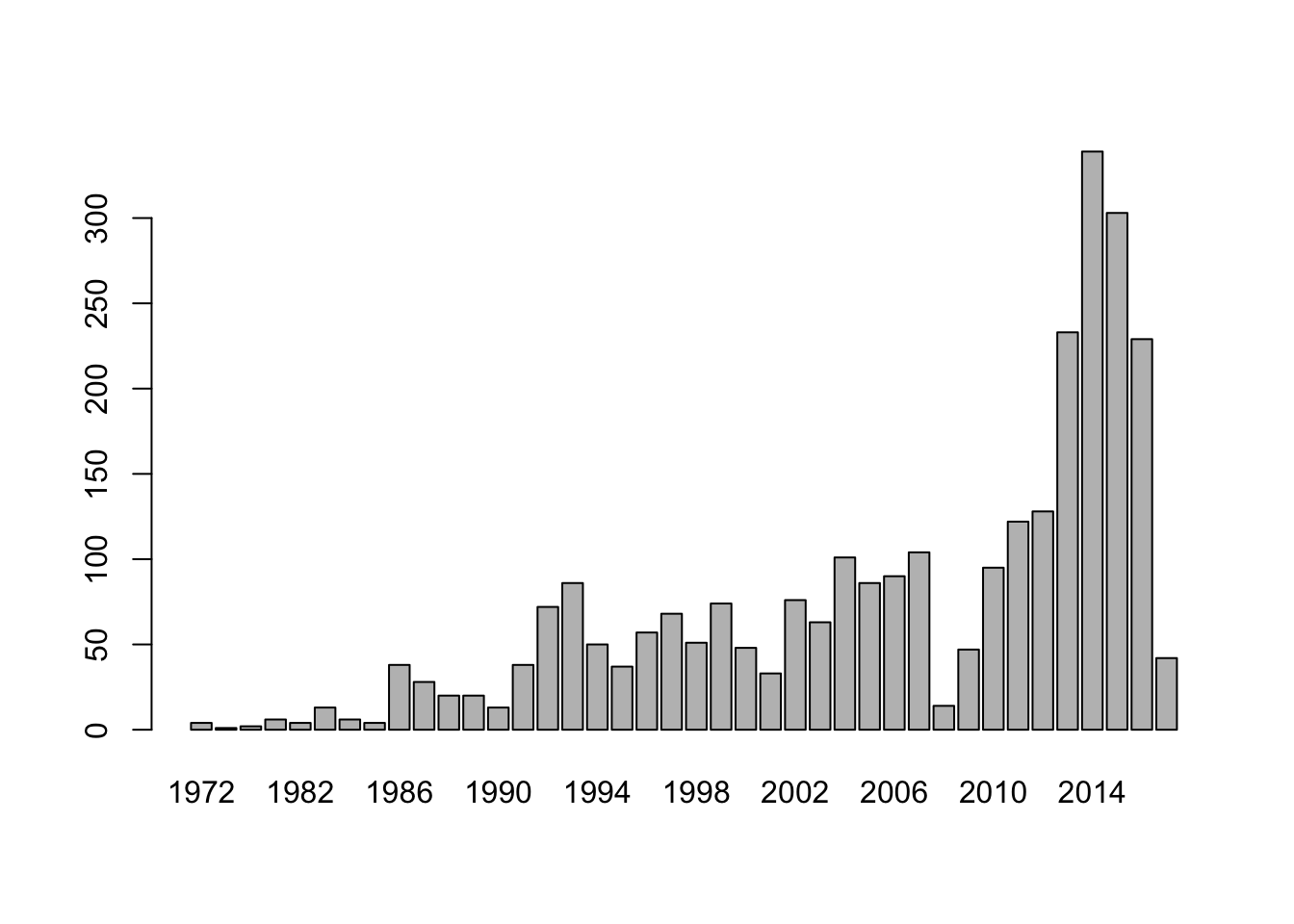
4.13 Bokeh plots
These are really nice looking but requires simple code. The “hover”" features make these plots especially appealing.
library(rbokeh)
p = figure(width=500,height=300) %>% ly_points(IPOyear,numIPO,data=res,hover=c(IPOyear,numIPO)) %>% ly_lines(IPOyear,numIPO,data=res)
p