Chapter 19 Zero or One: Optimal Digital Portfolios
This chapter is taken from the published paper “Digital Portfolios”, see S. Das (2013).
19.1 Digital Assets
Digital assets are investments with returns that are binary in nature, i.e., they either have a very large or very small payoff. We explore the features of optimal portfolios of digital assets such as venture investments, credit assets, search keyword groups, and lotteries. These portfolios comprise correlated assets with joint Bernoulli distributions. Using a simple, standard, fast recursion technique to generate the return distribution of the portfolio, we derive guidelines on how investors in digital assets may think about constructing their portfolios. We find that digital portfolios are better when they are homogeneous in the size of the assets, but heterogeneous in the success probabilities of the asset components.
The return distributions of digital portfolios are highly skewed and fat-tailed. A good example of such a portfolio is a venture fund. A simple representation of the payoff to a digital investment is Bernoulli with a large payoff for a successful outcome and a very small (almost zero) payoff for a failed one. The probability of success of digital investments is typically small, in the region of 5–25% for new ventures, see Sarin, Das, and Jagannathan (2003). Optimizing portfolios of such investments is therefore not amenable to standard techniques used for mean-variance optimization.
It is also not apparent that the intuitions obtained from the mean-variance setting carry over to portfolios of Bernoulli assets. For instance, it is interesting to ask, ceteris paribus, whether diversification by increasing the number of assets in the digital portfolio is always a good thing. Since Bernoulli portfolios involve higher moments, how diversification is achieved is by no means obvious. We may also ask whether it is preferable to include assets with as little correlation as possible or is there a sweet spot for the optimal correlation levels of the assets? Should all the investments be of even size, or is it preferable to take a few large bets and several small ones? And finally, is a mixed portfolio of safe and risky assets preferred to one where the probability of success is more uniform across assets? These are all questions that are of interest to investors in digital type portfolios, such as CDO investors, venture capitalists and investors in venture funds.
We will use a method that is based on standard recursion for modeling of the exact return distribution of a Bernoulli portfolio. This method on which we build was first developed by Andersen, Sidenius, and Basu (2003) for generating loss distributions of credit portfolios. We then examine the properties of these portfolios in a stochastic dominance framework framework to provide guidelines to digital investors. These guidelines are found to be consistent with prescriptions from expected utility optimization. The prescriptions are as follows:
- Holding all else the same, more digital investments are preferred, meaning for example, that a venture portfolio should seek to maximize market share.
- As with mean-variance portfolios, lower asset correlation is better, unless the digital investor’s payoff depends on the upper tail of returns.
- A strategy of a few large bets and many small ones is inferior to one with bets being roughly the same size.
- And finally, a mixed portfolio of low-success and high-success assets is better than one with all assets of the same average success probability level.
19.2 Modeling Digital Portfolios
Assume that the investor has a choice of \(n\) investments in digital assets (e.g., start-up firms). The investments are indexed \(i=1,2, \ldots, n\). Each investment has a probability of success that is denoted \(q_i\), and if successful, the payoff returned is \(S_i\) dollars. With probability \((1-q_i)\), the investment will not work out, the start-up will fail, and the money will be lost in totality. Therefore, the payoff (cashflow) is
\[ \mbox{Payoff} = C_i = \left\{ \begin{array}{cl} S_i & \mbox{with prob } q_i \\ 0 & \mbox{with prob } (1-q_i) \end{array} \right. \]
The specification of the investment as a Bernoulli trial is a simple representation of reality in the case of digital portfolios. This mimics well for example, the case of the venture capital business. Two generalizations might be envisaged. First, we might extend the model to allowing \(S_i\) to be random, i.e., drawn from a range of values. This will complicate the mathematics, but not add much in terms of enriching the model’s results. Second, the failure payoff might be non-zero, say an amount \(a_i\). Then we have a pair of Bernoulli payoffs \(\{S_i, a_i\}\). Note that we can decompose these investment payoffs into a project with constant payoff \(a_i\) plus another project with payoffs \(\{S_i-a_i,0\}\), the latter being exactly the original setting where the failure payoff is zero. Hence, the version of the model we solve in this note, with zero failure payoffs, is without loss of generality.
Unlike stock portfolios where the choice set of assets is assumed to be multivariate normal, digital asset investments have a joint Bernoulli distribution. Portfolio returns of these investments are unlikely to be Gaussian, and hence higher-order moments are likely to matter more. In order to generate the return distribution for the portfolio of digital assets, we need to account for the correlations across digital investments. We adopt the following simple model of correlation. Define \(y_i\) to be the performance proxy for the \(i\)-th asset. This proxy variable will be simulated for comparison with a threshold level of performance to determine whether the asset yielded a success or failure. It is defined by the following function, widely used in the correlated default modeling literature, see for example Andersen, Sidenius, and Basu (2003):
\[ y_i = \rho_i \; X + \sqrt{1-\rho_i^2}\; Z_i, \quad i = 1 \ldots n \]
where \(\rho_i \in [0,1]\) is a coefficient that correlates threshold \(y_i\) with a normalized common factor \(X \sim N(0,1)\). The common factor drives the correlations amongst the digital assets in the portfolio. We assume that \(Z_i \sim N(0,1)\) and \(\mbox{Corr}(X,Z_i)=0, \forall i\). Hence, the correlation between assets \(i\) and \(j\) is given by \(\rho_i \times \rho_j\). Note that the mean and variance of \(y_i\) are: \(E(y_i)=0, Var(y_i)=1, \forall i\). Conditional on \(X\), the values of \(y_i\) are all independent, as \(\mbox{Corr}(Z_i, Z_j)=0\).
We now formalize the probability model governing the success or failure of the digital investment. We define a variable \(x_i\), with distribution function \(F(\cdot)\), such that \(F(x_i) = q_i\), the probability of success of the digital investment. Conditional on a fixed value of \(X\), the probability of success of the \(i\)-th investment is defined as
\[ p_i^X \equiv Pr[y_i < x_i | X] \]
Assuming \(F\) to be the normal distribution function, we have
\[ \begin{align} p_i^X &= Pr \left[ \rho_i X + \sqrt{1-\rho_i^2}\; Z_i < x_i | X \right] \nonumber \\ &= Pr \left[ Z_i < \frac{x_i - \rho_i X}{\sqrt{1-\rho_i^2}} | X \right] \nonumber \\ &= \Phi \left[ \frac{F^{-1}(q_i) - \rho_i X}{\sqrt{1-\rho_i}} \right] \end{align} \]
where \(\Phi(.)\) is the cumulative normal density function. Therefore, given the level of the common factor \(X\), asset correlation \(\rho\), and the unconditional success probabilities \(q_i\), we obtain the conditional success probability for each asset \(p_i^X\). As \(X\) varies, so does \(p_i^X\). For the numerical examples here we choose the function \(F(x_i)\) to the cumulative normal probability function.
19.3 Fast Computation Approach
We use a fast technique for building up distributions for sums of Bernoulli random variables. In finance, this recursion technique was introduced in the credit portfolio modeling literature by Andersen, Sidenius, and Basu (2003).
We deem an investment in a digital asset as successful if it achieves its high payoff \(S_i\). The cashflow from the portfolio is a random variable \(C = \sum_{i=1}^n C_i\). The maximum cashflow that may be generated by the portfolio will be the sum of all digital asset cashflows, because each and every outcome was a success, i.e.,
\[ C_{max} = \sum_{i=1}^n \; S_i \]
To keep matters simple, we assume that each \(S_i\) is an integer, and that we round off the amounts to the nearest significant digit. So, if the smallest unit we care about is a million dollars, then each \(S_i\) will be in units of integer millions.
Recall that, conditional on a value of \(X\), the probability of success of digital asset \(i\) is given as \(p_i^X\). The recursion technique will allow us to generate the portfolio cashflow probability distribution for each level of \(X\). We will then simply compose these conditional (on \(X\)) distributions using the marginal distribution for \(X\), denoted \(g(X)\), into the unconditional distribution for the entire portfolio. Therefore, we define the probability of total cashflow from the portfolio, conditional on \(X\), to be \(f(C | X)\). Then, the unconditional cashflow distribution of the portfolio becomes
\[ f(C) = \int_X \; f(C | X) \cdot g(X)\; dX \quad \quad \quad (CONV) \]
The distribution \(f(C | X)\) is easily computed numerically as follows.
We index the assets with \(i=1 \ldots n\). The cashflow from all assets taken together will range from zero to \(C_{max}\). Suppose this range is broken into integer buckets, resulting in \(N_B\) buckets in total, each one containing an increasing level of total cashflow. We index these buckets by \(j=1 \ldots N_B\), with the cashflow in each bucket equal to \(B_j\). \(B_j\) represents the total cashflow from all assets (some pay off and some do not), and the buckets comprise the discrete support for the entire distribution of total cashflow from the portfolio. For example, suppose we had 10 assets, each with a payoff of \(C_i=3\). Then \(C_{max}=30\). A plausible set of buckets comprising the support of the cashflow distribution would be: \(\{0,3,6,9,12,15,18,21,24,27,C_{max}\}\).
Define \(P(k,B_j)\) as the probability of bucket \(j\)’s cashflow level \(B_j\) if we account for the first \(k\) assets. For example, if we had just 3 assets, with payoffs of value 1,3,2 respectively, then we would have 7 buckets, i.e. \(B_j=\{0,1,2,3,4,5,6\}\). After accounting for the first asset, the only possible buckets with positive probability would be \(B_j=0,1\), and after the first two assets, the buckets with positive probability would be \(B_j=0,1,3,4\). We begin with the first asset, then the second and so on, and compute the probability of seeing the returns in each bucket. Each probability is given by the following recursion:
\[ P(k+1,B_j) = P(k,B_j)\;[1-p^X_{k+1}] + P(k,B_j - S_{k+1}) \; p^X_{k+1}, \quad k = 1, \ldots, n-1. \quad \quad (REC) \]
Thus the probability of a total cashflow of \(B_j\) after considering the first \((k+1)\) firms is equal to the sum of two probability terms. First, the probability of the same cashflow \(B_j\) from the first \(k\) firms, given that firm \((k+1)\) did not succeed. Second, the probability of a cashflow of \(B_j - S_{k+1}\) from the first \(k\) firms and the \((k+1)\)-st firm does succeed.
We start off this recursion from the first asset, after which the \(N_B\) buckets are all of probability zero, except for the bucket with zero cashflow (the first bucket) and the one with \(S_1\) cashflow, i.e.,
\[ \begin{align} P(1,0) &= 1-p^X_1 \\ P(1,S_1) &= p^X_1 \end{align} \]
All the other buckets will have probability zero, i.e., \(P(1,B_j \neq \{0,S_1\})=0\). With these starting values, we can run the system up from the first asset to the \(n\)-th one by repeated application of equation (REC). Finally, we will have the entire distribution \(P(n,B_j)\), conditional on a given value of \(X\). We then compose all these distributions that are conditional on \(X\) into one single cashflow distribution using equation (CONV). This is done by numerically integrating over all values of \(X\).
library(pspline)
#Library for Digital Portfolio Analysis
#Copyright, Sanjiv Das, Dec 1, 2008.

#------------------------------------------------------------
#Function to implement the Andersen-Sidenius-Basu (Risk, 2003)
#recursion algorithm. Note that the probabilities are fixed,
#i.e. conditional on a given level of factor. The full blown
#distribution comes from the integral over all levels of the factor.
#INPUTS (example)
#w = c(1,7,3,2)             #Loss weights
#p = c(0.05, 0.2, 0.03, 0.1)    #Loss probabilities

asbrec = function(w,p) {

#BASIC SET UP
N = length(w)
maxloss = sum(w)
bucket = c(0,seq(maxloss))
LP = matrix(0,N,maxloss+1)      #probability grid over losses

#DO FIRST FIRM
LP[1,1] = 1-p[1];
LP[1,w[1]+1] = p[1];

#LOOP OVER REMAINING FIRMS
for (i in seq(2,N)) {
    for (j in seq(maxloss+1)) {
        LP[i,j] = LP[i-1,j]*(1-p[i])
        if (bucket[j]-w[i] >= 0) {
            LP[i,j] = LP[i,j] + LP[i-1,j-w[i]]*p[i]
        }
    }
}

#FINISH UP
lossprobs = LP[N,]
#print(t(LP))
#print(c("Sum of final probs = ",sum(lossprobs)))
result = matrix(c(bucket,lossprobs),(maxloss+1),2)
} #END ASBREC
We use this function in the following example.
#EXAMPLE
w = c(1,7,3,2)
p = c(0.05, 0.2, 0.03, 0.1)
res = asbrec(w,p)
print(res)
## [,1] [,2]
## [1,] 0 0.66348
## [2,] 1 0.03492
## [3,] 2 0.07372
## [4,] 3 0.02440
## [5,] 4 0.00108
## [6,] 5 0.00228
## [7,] 6 0.00012
## [8,] 7 0.16587
## [9,] 8 0.00873
## [10,] 9 0.01843
## [11,] 10 0.00610
## [12,] 11 0.00027
## [13,] 12 0.00057
## [14,] 13 0.00003barplot(res[,2],names.arg=res[,1],col=2)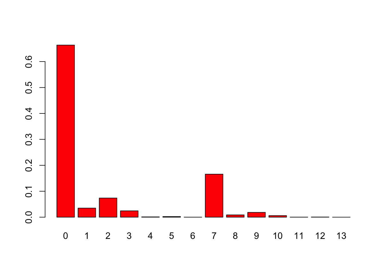
Here is a second example. Here each column represents one pass through the recursion. Since there are five assets, we get five passes, and the final column is the result we are looking for.
#EXAMPLE
w = c(5,8,4,2,1)
p = array(1/length(w),length(w))
res = asbrec(w,p)
print(res)
## [,1] [,2]
## [1,] 0 0.32768
## [2,] 1 0.08192
## [3,] 2 0.08192
## [4,] 3 0.02048
## [5,] 4 0.08192
## [6,] 5 0.10240
## [7,] 6 0.04096
## [8,] 7 0.02560
## [9,] 8 0.08704
## [10,] 9 0.04096
## [11,] 10 0.02560
## [12,] 11 0.01024
## [13,] 12 0.02176
## [14,] 13 0.02560
## [15,] 14 0.01024
## [16,] 15 0.00640
## [17,] 16 0.00128
## [18,] 17 0.00512
## [19,] 18 0.00128
## [20,] 19 0.00128
## [21,] 20 0.00032barplot(res[,2],names.arg=res[,1],col=2)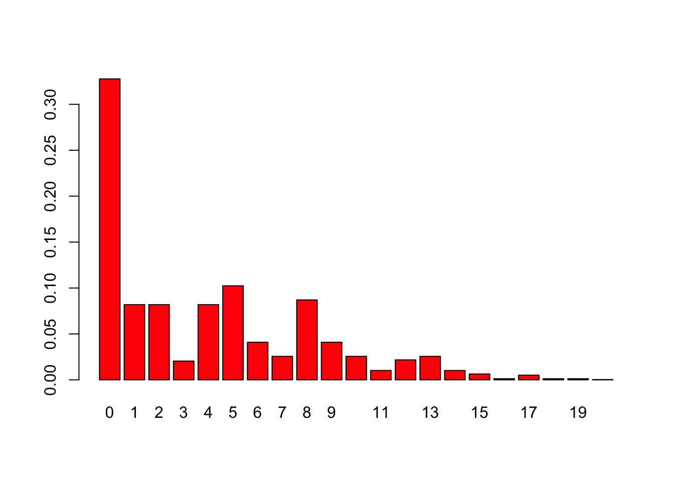
We can explore these recursion calculations in some detail as follows. Note that in our example \(p_i = 0.2, i = 1,2,3,4,5\). We are interested in computing \(P(k,B)\), where \(k\) denotes the \(k\)-th recursion pass, and \(B\) denotes the return bucket. Recall that we have five assets with return levels of \(\{5,8,4,2,1\}\), respecitvely. After \(i=1\), we have
\[ \begin{align} P(1,0) &= (1-p_1) = 0.8\\ P(1,5) &= p_1 = 0.2\\ P(1,j) &= 0, j \neq \{0,5\} \end{align} \]
The completes the first recursion pass and the values can be verified from the R output above by examining column 2 (column 1 contains the values of the return buckets). We now move on the calculations needed for the second pass in the recursion.
\[ \begin{align} P(2,0) &= P(1,0)(1-p_2) = 0.64\\ P(2,5) &= P(1,5)(1-p_2) + P(1,5-8) p_2 = 0.2 (0.8) + 0 (0.2) = 0.16\\ P(2,8) &= P(1,8) (1-p_2) + P(1,8-8) p_2 = 0 (0.8) + 0.8 (0.2) = 0.16\\ P(2,13) &= P(1,13)(1-p_2) + P(1,13-8) p_2 = 0 (0.8) + 0.2 (0.2) = 0.04\\ P(2,j) &= 0, j \neq \{0,5,8,13\} \end{align} \]
The third recursion pass is as follows:
\[ \begin{align} P(3,0) &= P(2,0)(1-p_3) = 0.512\\ P(3,4) &= P(2,4)(1-p_3) + P(2,4-4) = 0(0.8) + 0.64(0.2) = 0.128\\ P(3,5) &= P(2,5)(1-p_3) + P(2,5-4) p_3 = 0.16 (0.8) + 0 (0.2) = 0.128\\ P(3,8) &= P(2,8) (1-p_3) + P(2,8-4) p_3 = 0.16 (0.8) + 0 (0.2) = 0.128\\ P(3,9) &= P(2,9) (1-p_3) + P(2,9-4) p_3 = 0 (0.8) + 0.16 (0.2) = 0.032\\ P(3,12) &= P(2,12) (1-p_3) + P(2,12-4) p_3 = 0 (0.8) + 0.16 (0.2) = 0.032\\ P(3,13) &= P(2,13) (1-p_3) + P(2,13-4) p_3 = 0.04 (0.8) + 0 (0.2) = 0.032\\ P(3,17) &= P(2,17) (1-p_3) + P(2,17-4) p_3 = 0 (0.8) + 0.04 (0.2) = 0.008\\ P(3,j) &= 0, j \neq \{0,4,5,8,9,12,13,17\} \end{align} \]
Note that the same computation work even when the outcomes are not of equal probability. Let’s do one more example.
#ONE FINAL EXAMPLE
#----------MAIN CALLING SEGMENT------------------
w = c(5,2,4,2,8,1,9)
p = array(0.2,length(w))
res = asbrec(w,p)
print(res)
## [,1] [,2]
## [1,] 0 0.2097152
## [2,] 1 0.0524288
## [3,] 2 0.1048576
## [4,] 3 0.0262144
## [5,] 4 0.0655360
## [6,] 5 0.0688128
## [7,] 6 0.0393216
## [8,] 7 0.0327680
## [9,] 8 0.0622592
## [10,] 9 0.0827392
## [11,] 10 0.0434176
## [12,] 11 0.0393216
## [13,] 12 0.0245760
## [14,] 13 0.0344064
## [15,] 14 0.0272384
## [16,] 15 0.0180224
## [17,] 16 0.0106496
## [18,] 17 0.0198656
## [19,] 18 0.0086016
## [20,] 19 0.0092160
## [21,] 20 0.0036864
## [22,] 21 0.0047104
## [23,] 22 0.0045568
## [24,] 23 0.0025088
## [25,] 24 0.0020480
## [26,] 25 0.0006144
## [27,] 26 0.0010752
## [28,] 27 0.0002560
## [29,] 28 0.0004096
## [30,] 29 0.0001024
## [31,] 30 0.0000512
## [32,] 31 0.0000128print(sum(res[,2]))## [1] 1barplot(res[,2],names.arg=res[,1],col=4)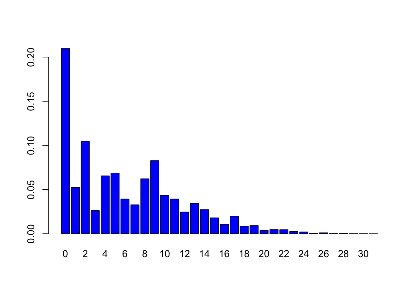
19.4 Combining conditional distributions
We now demonstrate how we will integrate the conditional probability distributions \(p^X\) into an unconditional probability distribution of outcomes, denoted
\[ p = \int_X p^X g(X) \; dX, \]
where \(g(X)\) is the density function of the state variable \(X\). We create a function to combine the conditional distribution functions. This function calls the asbrec function that we had used earlier.
#---------------------------
#FUNCTION TO COMPUTE FULL RETURN DISTRIBUTION
#INTEGRATES OVER X BY CALLING ASBREC.R
digiprob = function(L,q,rho) {  #Note: L,q same as w,p from before
    dx = 0.1
    x = seq(-40,40)*dx
    fx = dnorm(x)*dx
    fx = fx/sum(fx)
    maxloss = sum(L)
    bucket = c(0,seq(maxloss))
    totp = array(0,(maxloss+1))
    for (i in seq(length(x))) {
        p = pnorm((qnorm(q)-rho*x[i])/sqrt(1-rho^2))
        ldist = asbrec(L,p)
        totp = totp + ldist[,2]*fx[i]
    }
    result = matrix(c(bucket,totp),(maxloss+1),2)
}
Note that now we will use the unconditional probabilities of success for each asset, and correlate them with a specified correlation level. We run this with two correlation levels \(\{-0.5, +0.5\}\).
#------INTEGRATE OVER CONDITIONAL DISTRIBUTIONS----
w = c(5,8,4,2,1)
q = c(0.1,0.2,0.1,0.05,0.15)
rho = 0.25
res1 = digiprob(w,q,rho)
rho = 0.75
res2 = digiprob(w,q,rho)
par(mfrow=c(2,1))
barplot(res1[,2],names.arg=res1[,1],xlab="portfolio value",
    ylab="probability",main="rho = 0.25")
barplot(res2[,2],names.arg=res2[,1],xlab="portfolio value",
    ylab="probability",main="rho = 0.75")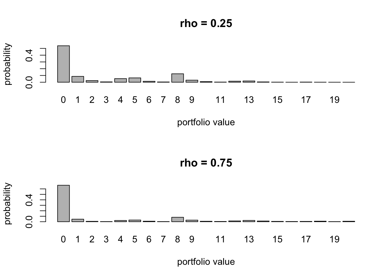
cbind(res1,res2)## [,1] [,2] [,3] [,4]
## [1,] 0 0.5391766174 0 0.666318464
## [2,] 1 0.0863707325 1 0.046624312
## [3,] 2 0.0246746918 2 0.007074104
## [4,] 3 0.0049966420 3 0.002885901
## [5,] 4 0.0534700675 4 0.022765422
## [6,] 5 0.0640540228 5 0.030785967
## [7,] 6 0.0137226107 6 0.009556413
## [8,] 7 0.0039074039 7 0.002895774
## [9,] 8 0.1247287209 8 0.081172499
## [10,] 9 0.0306776806 9 0.029154885
## [11,] 10 0.0086979993 10 0.008197488
## [12,] 11 0.0021989842 11 0.004841742
## [13,] 12 0.0152035638 12 0.014391319
## [14,] 13 0.0186144920 13 0.023667222
## [15,] 14 0.0046389439 14 0.012776165
## [16,] 15 0.0013978502 15 0.006233366
## [17,] 16 0.0003123473 16 0.004010559
## [18,] 17 0.0022521668 17 0.005706283
## [19,] 18 0.0006364672 18 0.010008267
## [20,] 19 0.0002001003 19 0.002144265
## [21,] 20 0.0000678949 20 0.008789582The left column of probabilities has correlation of \(\rho=0.25\) and the right one is the case when \(\rho=0.75\). We see that the probabilities on the right are lower for low outcomes (except zero) and high for high outcomes. Why?
19.5 Stochastic Dominance (SD)
SD is an ordering over probabilistic bundles. We may want to know if one VC’s portfolio dominates another in a risk-adjusted sense. Different SD concepts apply to answer this question. For example if portfolio \(A\) does better than portfolio \(B\) in every state of the world, it clearly dominates. This is called state-by-state dominance, and is hardly ever encountered. Hence, we briefly examine two more common types of SD.
- First-order Stochastic Dominance (FSD): For cumulative distribution function \(F(X)\) over states \(X\), portfolio \(A\) dominates \(B\) if \(\mbox{Prob}(A \geq k) \geq \mbox{Prob}(B \geq k)\) for all states \(k \in X\), and \(\mbox{Prob}(A \geq k) > \mbox{Prob}(B \geq k)\) for some \(k\). It is the same as \(\mbox{Prob}(A \leq k) \leq \mbox{Prob}(B \leq k)\) for all states \(k \in X\), and \(\mbox{Prob}(A \leq k) < \mbox{Prob}(B \leq k)\) for some \(k\).This implies that \(F_A(k) \leq F_B(k)\). The mean outcome under \(A\) will be higher than under \(B\), and all increasing utility functions will give higher utility for \(A\). This is a weaker notion of dominance than state-wise, but also not as often encountered in practice.
- Second-order Stochastic Dominance (SSD): Here the portfolios have the same mean but the risk is less for portfolio \(A\). Then we say that portfolio \(A\) has a mean-preserving spread over portfolio \(B\). Technically this is the same as \(\int_{-\infty}^k [F_A(k) - F_B(k)] \; dX < 0\), and \(\int_X X dF_A(X) = \int_X X dF_B(X)\). Mean-variance models in which portfolios on the efficient frontier dominate those below are a special case of SSD. See the example below, there is no FSD, but there is SSD.
#FIRST_ORDER SD
x = seq(-4,4,0.1)
F_B = pnorm(x,mean=0,sd=1);
F_A = pnorm(x,mean=0.25,sd=1);
F_A-F_B   #FSD exists
## [1] -2.098272e-05 -3.147258e-05 -4.673923e-05 -6.872414e-05 -1.000497e-04
## [6] -1.442118e-04 -2.058091e-04 -2.908086e-04 -4.068447e-04 -5.635454e-04
## [11] -7.728730e-04 -1.049461e-03 -1.410923e-03 -1.878104e-03 -2.475227e-03
## [16] -3.229902e-03 -4.172947e-03 -5.337964e-03 -6.760637e-03 -8.477715e-03
## [21] -1.052566e-02 -1.293895e-02 -1.574810e-02 -1.897740e-02 -2.264252e-02
## [26] -2.674804e-02 -3.128519e-02 -3.622973e-02 -4.154041e-02 -4.715807e-02
## [31] -5.300548e-02 -5.898819e-02 -6.499634e-02 -7.090753e-02 -7.659057e-02
## [36] -8.191019e-02 -8.673215e-02 -9.092889e-02 -9.438507e-02 -9.700281e-02
## [41] -9.870633e-02 -9.944553e-02 -9.919852e-02 -9.797262e-02 -9.580405e-02
## [46] -9.275614e-02 -8.891623e-02 -8.439157e-02 -7.930429e-02 -7.378599e-02
## [51] -6.797210e-02 -6.199648e-02 -5.598646e-02 -5.005857e-02 -4.431528e-02
## [56] -3.884257e-02 -3.370870e-02 -2.896380e-02 -2.464044e-02 -2.075491e-02
## [61] -1.730902e-02 -1.429235e-02 -1.168461e-02 -9.458105e-03 -7.580071e-03
## [66] -6.014807e-03 -4.725518e-03 -3.675837e-03 -2.831016e-03 -2.158775e-03
## [71] -1.629865e-03 -1.218358e-03 -9.017317e-04 -6.607827e-04 -4.794230e-04
## [76] -3.443960e-04 -2.449492e-04 -1.724935e-04 -1.202675e-04 -8.302381e-05
## [81] -5.674604e-05#SECOND_ORDER SD
x = seq(-4,4,0.1)
F_B = pnorm(x,mean=0,sd=2);
F_A = pnorm(x,mean=0,sd=1);
print(F_A-F_B) #No FSD## [1] -0.02271846 -0.02553996 -0.02864421 -0.03204898 -0.03577121
## [6] -0.03982653 -0.04422853 -0.04898804 -0.05411215 -0.05960315
## [11] -0.06545730 -0.07166345 -0.07820153 -0.08504102 -0.09213930
## [16] -0.09944011 -0.10687213 -0.11434783 -0.12176261 -0.12899464
## [21] -0.13590512 -0.14233957 -0.14812981 -0.15309708 -0.15705611
## [26] -0.15982015 -0.16120699 -0.16104563 -0.15918345 -0.15549363
## [31] -0.14988228 -0.14229509 -0.13272286 -0.12120570 -0.10783546
## [36] -0.09275614 -0.07616203 -0.05829373 -0.03943187 -0.01988903
## [41] 0.00000000 0.01988903 0.03943187 0.05829373 0.07616203
## [46] 0.09275614 0.10783546 0.12120570 0.13272286 0.14229509
## [51] 0.14988228 0.15549363 0.15918345 0.16104563 0.16120699
## [56] 0.15982015 0.15705611 0.15309708 0.14812981 0.14233957
## [61] 0.13590512 0.12899464 0.12176261 0.11434783 0.10687213
## [66] 0.09944011 0.09213930 0.08504102 0.07820153 0.07166345
## [71] 0.06545730 0.05960315 0.05411215 0.04898804 0.04422853
## [76] 0.03982653 0.03577121 0.03204898 0.02864421 0.02553996
## [81] 0.02271846cumsum(F_A-F_B)## [1] -2.271846e-02 -4.825842e-02 -7.690264e-02 -1.089516e-01 -1.447228e-01
## [6] -1.845493e-01 -2.287779e-01 -2.777659e-01 -3.318781e-01 -3.914812e-01
## [11] -4.569385e-01 -5.286020e-01 -6.068035e-01 -6.918445e-01 -7.839838e-01
## [16] -8.834239e-01 -9.902961e-01 -1.104644e+00 -1.226407e+00 -1.355401e+00
## [21] -1.491306e+00 -1.633646e+00 -1.781776e+00 -1.934873e+00 -2.091929e+00
## [26] -2.251749e+00 -2.412956e+00 -2.574002e+00 -2.733185e+00 -2.888679e+00
## [31] -3.038561e+00 -3.180856e+00 -3.313579e+00 -3.434785e+00 -3.542620e+00
## [36] -3.635376e+00 -3.711538e+00 -3.769832e+00 -3.809264e+00 -3.829153e+00
## [41] -3.829153e+00 -3.809264e+00 -3.769832e+00 -3.711538e+00 -3.635376e+00
## [46] -3.542620e+00 -3.434785e+00 -3.313579e+00 -3.180856e+00 -3.038561e+00
## [51] -2.888679e+00 -2.733185e+00 -2.574002e+00 -2.412956e+00 -2.251749e+00
## [56] -2.091929e+00 -1.934873e+00 -1.781776e+00 -1.633646e+00 -1.491306e+00
## [61] -1.355401e+00 -1.226407e+00 -1.104644e+00 -9.902961e-01 -8.834239e-01
## [66] -7.839838e-01 -6.918445e-01 -6.068035e-01 -5.286020e-01 -4.569385e-01
## [71] -3.914812e-01 -3.318781e-01 -2.777659e-01 -2.287779e-01 -1.845493e-01
## [76] -1.447228e-01 -1.089516e-01 -7.690264e-02 -4.825842e-02 -2.271846e-02
## [81] 1.353084e-1619.6 Portfolio Characteristics
Armed with this established machinery, there are several questions an investor (e.g. a VC) in a digital portfolio may pose. First, is there an optimal number of assets, i.e., ceteris paribus, are more assets better than fewer assets, assuming no span of control issues? Second, are Bernoulli portfolios different from mean-variances ones, in that is it always better to have less asset correlation than more correlation? Third, is it better to have an even weighting of investment across the assets or might it be better to take a few large bets amongst many smaller ones? Fourth, is a high dispersion of probability of success better than a low dispersion? These questions are very different from the ones facing investors in traditional mean-variance portfolios. We shall examine each of these questions in turn.
19.7 How many assets?
With mean-variance portfolios, keeping the mean return of the portfolio fixed, more securities in the portfolio is better, because diversification reduces the variance of the portfolio. Also, with mean-variance portfolios, higher-order moments do not matter. But with portfolios of Bernoulli assets, increasing the number of assets might exacerbate higher-order moments, even though it will reduce variance. Therefore it may not be worthwhile to increase the number of assets (\(n\)) beyond a point.
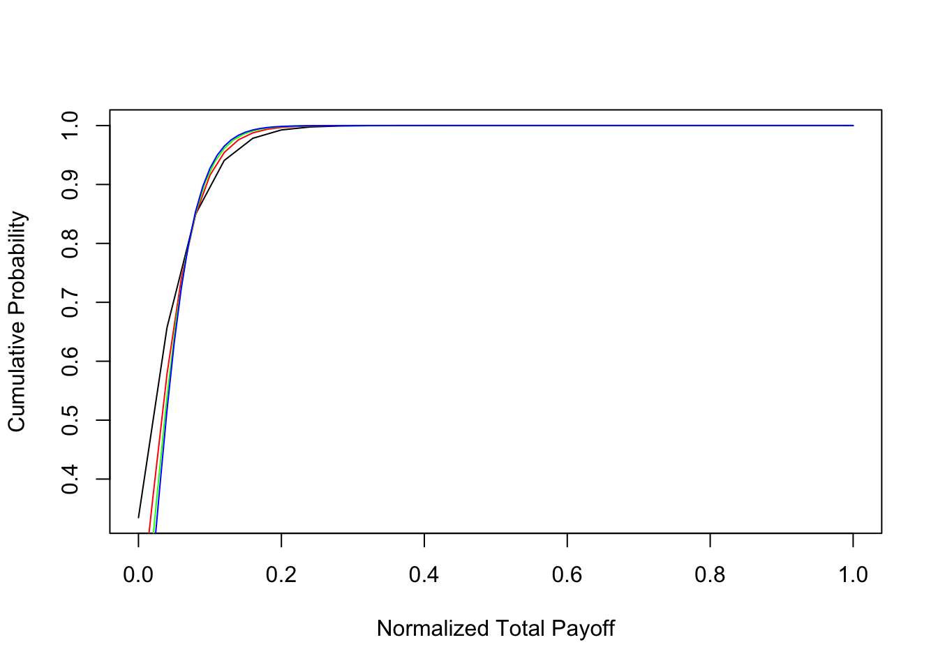
In order to assess this issue we conducted the following experiment. We invested in \(n\) assets each with payoff of \(1/n\). Hence, if all assets succeed, the total (normalized) payoff is 1. This normalization is only to make the results comparable across different \(n\), and is without loss of generality. We also assumed that the correlation parameter is \(\rho_i = 0.25\), for all \(i\). To make it easy to interpret the results, we assumed each asset to be identical with a success probability of \(q_i=0.05\) for all \(i\). Using the recursion technique, we computed the probability distribution of the portfolio payoff for four values of \(n = \{25,50,75,100\}\). The distribution function is plotted below. There are 4 plots, one for each \(n\), and if we look at the bottom left of the plot, the leftmost line is for \(n=100\). The next line to the right is for \(n=75\), and so on.
One approach to determining if greater \(n\) is better for a digital portfolio is to investigate if a portfolio of \(n\) assets stochastically dominates one with less than \(n\) assets. On examination of the shapes of the distribution functions for different \(n\), we see that it is likely that as \(n\) increases, we obtain portfolios that exhibit second-order stochastic dominance (SSD) over portfolios with smaller \(n\). The return distribution when \(n=100\) (denoted \(G_{100}\)) would dominate that for \(n=25\) (denoted \(G_{25}\)) in the SSD sense, if \(\int_x x \; dG_{100}(x) = \int_x x \; dG_{25}(x)\), and \(\int_0^u [G_{100}(x) - G_{25}(x)]\; dx \leq 0\) for all \(u \in (0,1)\). That is, \(G_{25}\) has a mean-preserving spread over \(G_{100}\), or \(G_{100}\) has the same mean as \(G_{25}\) but lower variance, i.e., implies superior mean-variance efficiency. To show this we plotted the integral \(\int_0^u [G_{100}(x) - G_{25}(x)] \; dx\) and checked the SSD condition. We found that this condition is satisfied (see Figure ). As is known, SSD implies mean-variance efficiency as well.
We also examine if higher \(n\) portfolios are better for a power utility investor with utility function, \(U(C) = \frac{(0.1 + C)^{1-\gamma}}{1-\gamma}\), where \(C\) is the normalized total payoff of the Bernoulli portfolio. Expected utility is given by \(\sum_C U(C)\; f(C)\). We set the risk aversion coefficient to \(\gamma=3\) which is in the standard range in the asset-pricing literature. The cpde below reports the results. We can see that the expected utility increases monotonically with \(n\). Hence, for a power utility investor, having more assets is better than less, keeping the mean return of the portfolio constant. Economically, in the specific case of VCs, this highlights the goal of trying to capture a larger share of the number of available ventures. The results from the SSD analysis are consistent with those of expected power utility.
#CHECK WHAT HAPPENS WHEN NUMBER OF ASSETS/ISSUERS INCREASES
#Result: No ordering with SSD, utility better with more names
#source("number_names.R")
#SECOND-ORDER STOCH DOMINANCE (SSD): GREATER num_names IS BETTER
num_names = c(25,50,75,100)
each_loss = 1
each_prob = 0.05
rho = 0.5^2
gam = 3

for (j in seq(4)) {
    L = array(each_loss,num_names[j])
    q = array(each_prob,num_names[j])
    res = digiprob(L,q,rho)
    rets = res[,1]/num_names[j]
    probs = res[,2]
    cumprobs = array(0,length(res[,2]))
    cumprobs[1] = probs[1]
    for (k in seq(2,length(res[,2]))) {
        cumprobs[k] = cumprobs[k-1] + probs[k]
    }
    if (j==1) {
        plot(rets,cumprobs,type="l",xlab="Normalized Total Payoff",ylab="Cumulative Probability")
        rets1 = rets
        cumprobs1 = cumprobs
        utility = sum(((0.1+rets)^(1-gam)/(1-gam))*probs)
    }
    if (j==2) {
        lines(rets,cumprobs,type="l",col="Red")
        utility = sum(((0.1+rets)^(1-gam)/(1-gam))*probs)
    }
    if (j==3) {
        lines(rets,cumprobs,type="l",col="Green")
        utility = sum(((0.1+rets)^(1-gam)/(1-gam))*probs)
    }
    if (j==4) {
        lines(rets,cumprobs,type="l",col="Blue")
        rets4 = rets
        cumprobs4 = cumprobs
        utility = sum(((0.1+rets)^(1-gam)/(1-gam))*probs)
    }
    mn = sum(rets*probs)
    idx = which(rets>0.03); p03 = sum(probs[idx])
    idx = which(rets>0.07); p07 = sum(probs[idx])
    idx = which(rets>0.10); p10 = sum(probs[idx])
    idx = which(rets>0.15); p15 = sum(probs[idx])
    print(c(mn,p03,p07,p10,p15))
    print(c("Utility = ",utility))
}
## [1] 0.04999545 0.66546862 0.34247245 0.15028422 0.05924270
## [1] "Utility = "        "-29.2593289535026"
## [1] 0.04999545 0.63326734 0.25935510 0.08448287 0.02410500
## [1] "Utility = "        "-26.7549907254343"
## [1] 0.04999545 0.61961559 0.22252474 0.09645862 0.01493276
## [1] "Utility = "        "-25.8764941625812"
## [1] 0.04999545 0.61180443 0.20168330 0.07267614 0.01109592
## [1] "Utility = "       "-25.433466221872"
We now look at stochastic dominance.
#PLOT DIFFERENCE IN DISTRIBUTION FUNCTIONS
#IF POSITIVE FLAT WEIGHTS BETTER THAN RISING WEIGHTS

fit = sm.spline(rets1,cumprobs1)
cumprobs1 = predict(fit,rets4)
plot(rets4,cumprobs1-matrix(cumprobs4),type="l",xlab="Normalized total payoff",ylab="Difference in cumulative probs")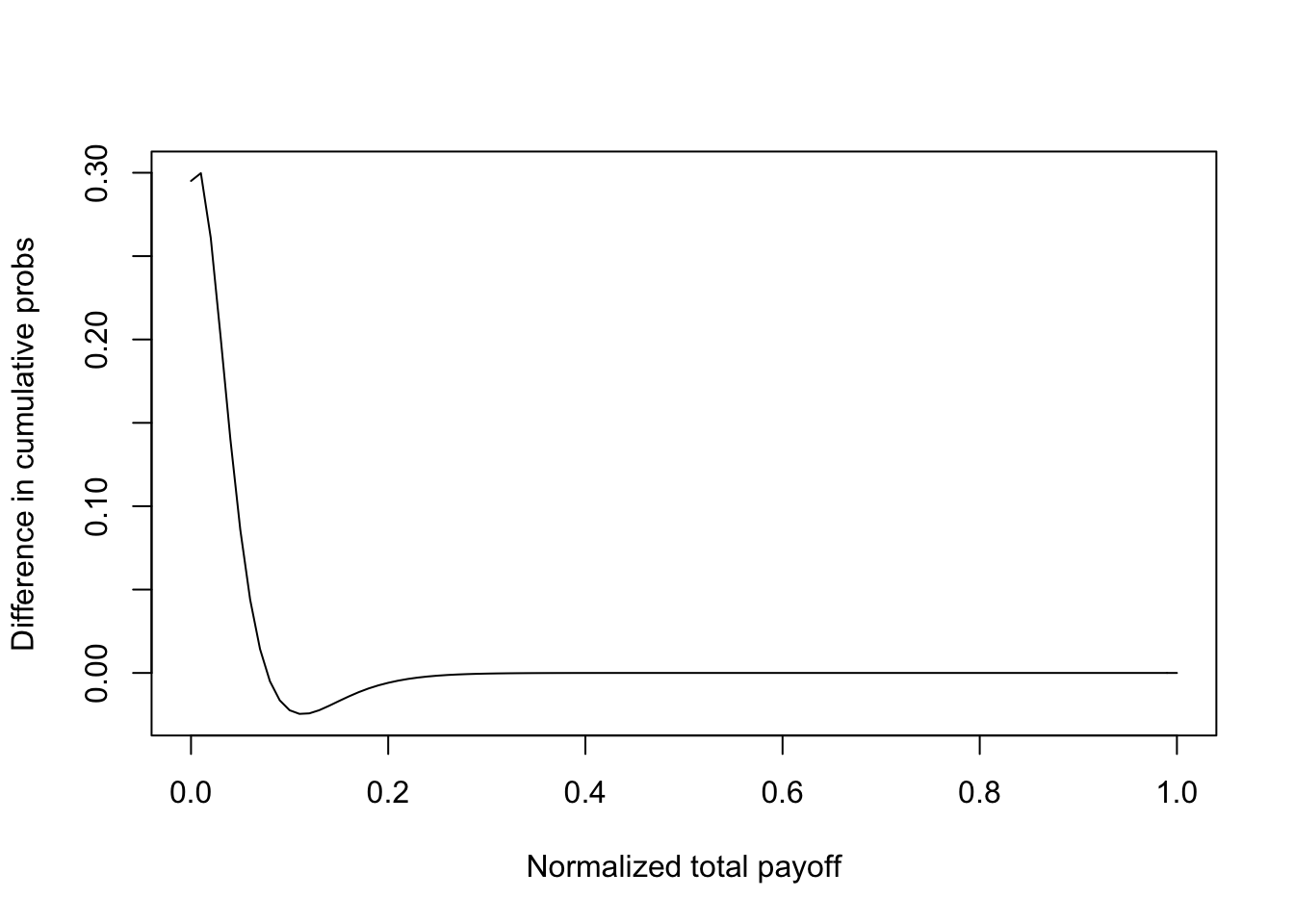
#CHECK IF SSD IS SATISFIED
#A SSD> B, if E(A)=E(B), and integral_0^y (F_A(z)-F_B(z)) dz <= 0, for all y
cumprobs4 = matrix(cumprobs4,length(cumprobs4),1)
n = length(cumprobs1)
ssd = NULL
for (j in 1:n) {
    check = sum(cumprobs4[1:j]-cumprobs1[1:j])
    ssd = c(ssd,check)
}
print(c("Max ssd = ",max(ssd)))  #If <0, then SSD satisfied, and it implies MV efficiency.
## [1] "Max ssd = " "-0.295083435837737"plot(rets4,ssd,type="l",xlab="Normalized total payoff",ylab="Integrated F(G100) minus F(G25)")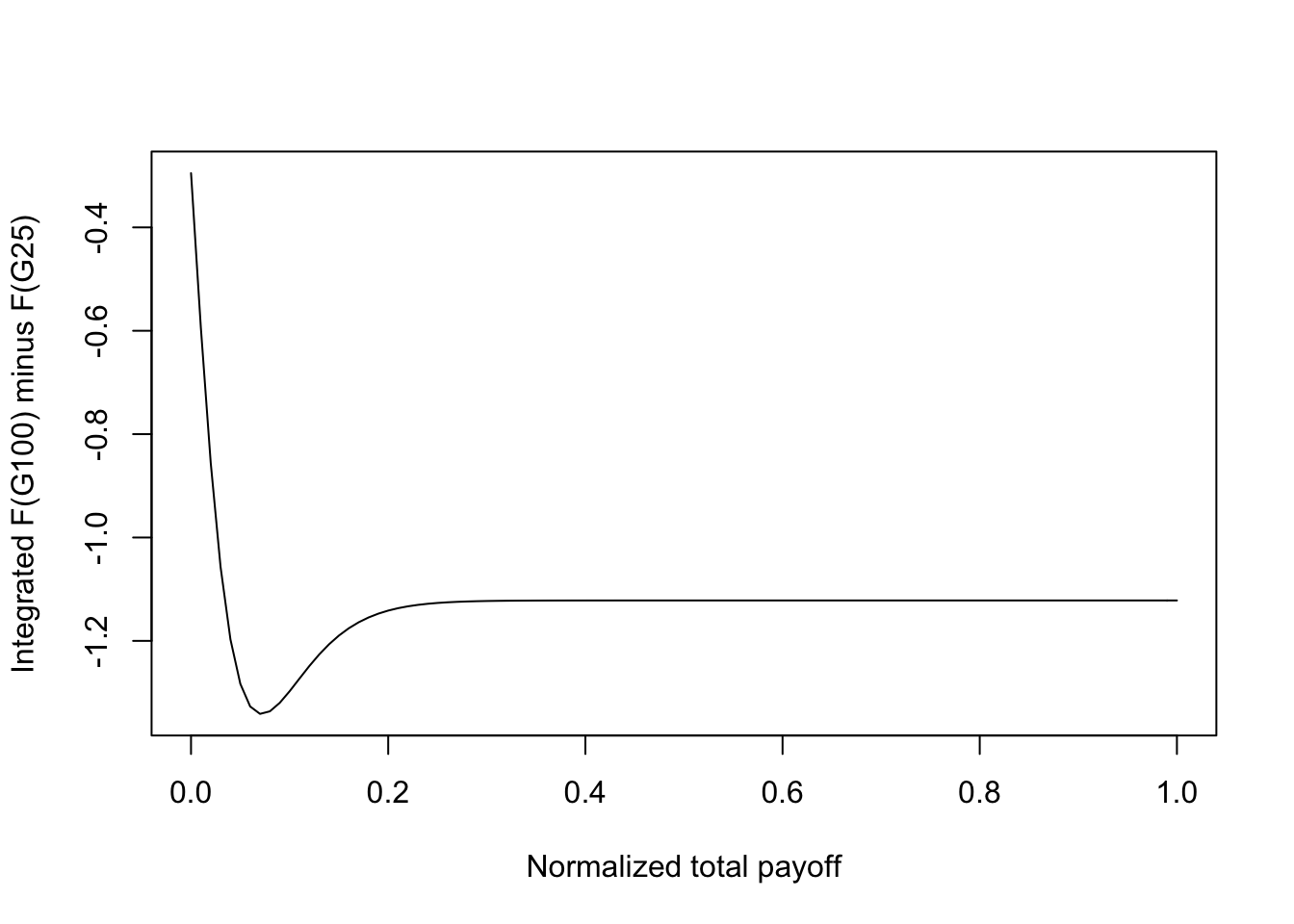
19.8 The impact of correlation
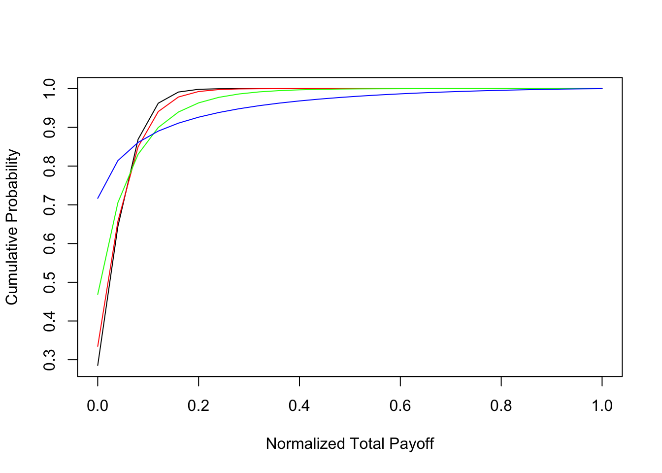
As with mean-variance portfolios, we expect that increases in payoff correlation for Bernoulli assets will adversely impact portfolios. In order to verify this intuition we analyzed portfolios keeping all other variables the same, but changing correlation. In the previous subsection, we set the parameter for correlation to be \(\rho = 0.25\). Here, we examine four levels of the correlation parameter: \(\rho=\{0.09, 0.25, 0.49, 0.81\}\). For each level of correlation, we computed the normalized total payoff distribution. The number of assets is kept fixed at \(n=25\) and the probability of success of each digital asset is \(0.05\) as before.
The results are shown in the Figures below where the probability distribution function of payoffs is shown for all four correlation levels. We find that the SSD condition is met, i.e., that lower correlation portfolios stochastically dominate (in the SSD sense) higher correlation portfolios. We also examined changing correlation in the context of a power utility investor with the same utility function as in the previous subsection. See results from the code below. We confirm that, as with mean-variance portfolios, Bernoulli portfolios also improve if the assets have low correlation. Hence, digital investors should also optimally attempt to diversify their portfolios. Insurance companies are a good example—they diversify risk across geographical and other demographic divisions.
#CHECK WHAT HAPPENS WHEN RHO INCREASES
#Result: No ordering with SSD, Lower rho is better in the utility metric
#source("change_rho.R")
num_names = 25
each_loss = 1
each_prob = 0.05
rho = c(0.3,0.5,0.7,0.9)^2
gam = 3

for (j in seq(4)) {
    L = array(each_loss,num_names)
    q = array(each_prob,num_names)
    res = digiprob(L,q,rho[j])
    rets = res[,1]/num_names
    probs = res[,2]
    cumprobs = array(0,length(res[,2]))
    cumprobs[1] = probs[1]
    for (k in seq(2,length(res[,2]))) {
        cumprobs[k] = cumprobs[k-1] + probs[k]
    }
    if (j==1) {
        plot(rets,cumprobs,type="l",xlab="Normalized Total Payoff",ylab="Cumulative Probability")
        cumprobs1 = cumprobs
        utility = sum(((0.1+rets)^(1-gam)/(1-gam))*probs)
    }
    if (j==2) {
        lines(rets,cumprobs,type="l",col="Red")
        utility = sum(((0.1+rets)^(1-gam)/(1-gam))*probs)
    }
    if (j==3) {
        lines(rets,cumprobs,type="l",col="Green")
        utility = sum(((0.1+rets)^(1-gam)/(1-gam))*probs)
    }
    if (j==4) {
        lines(rets,cumprobs,type="l",col="Blue")
        cumprobs2 = cumprobs
        utility = sum(((0.1+rets)^(1-gam)/(1-gam))*probs)
    }
    mn = sum(rets*probs)
    idx = which(rets>0.03); p03 = sum(probs[idx])
    idx = which(rets>0.07); p07 = sum(probs[idx])
    idx = which(rets>0.10); p10 = sum(probs[idx])
    idx = which(rets>0.15); p15 = sum(probs[idx])
    print(c(mn,p03,p07,p10,p15))
    print(c("Utility = ",utility))
}
## [1] 0.04999940 0.71474772 0.35589301 0.13099315 0.03759002
## [1] "Utility = "        "-28.1122419295505"
## [1] 0.04999545 0.66546862 0.34247245 0.15028422 0.05924270
## [1] "Utility = "        "-29.2593289535026"
## [1] 0.04998484 0.53141370 0.29432093 0.16957177 0.10034508
## [1] "Utility = "        "-32.6682122683527"
## [1] 0.04997715 0.28323169 0.18573188 0.13890452 0.10963643
## [1] "Utility = "        "-39.7578637369197"
19.9 Uneven bets?
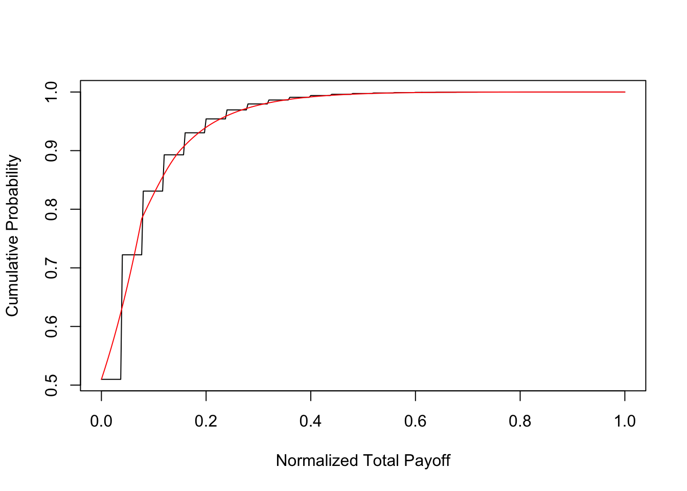
Digital asset investors are often faced with the question of whether to bet even amounts across digital investments, or to invest with different weights. We explore this question by considering two types of Bernoulli portfolios. Both have \(n=25\) assets within them, each with a success probability of \(q_i=0.05\). The first has equal payoffs, i.e., \(1/25\) each. The second portfolio has payoffs that monotonically increase, i.e., the payoffs are equal to \(j/325, j=1,2,\ldots,25\). We note that the sum of the payoffs in both cases is 1. The code output shows the utility of the investor, where the utility function is the same as in the previous sections. We see that the utility for the balanced portfolio is higher than that for the imbalanced one. Also the balanced portfolio evidences SSD over the imbalanced portfolio. However, the return distribution has fatter tails when the portfolio investments are imbalanced. Hence, investors seeking to distinguish themselves by taking on greater risk in their early careers may be better off with imbalanced portfolios.
#PLOT DIFFERENCE IN DISTRIBUTION FUNCTIONS
#IF POSITIVE FLAT WEIGHTS BETTER THAN RISING WEIGHTS
plot(rets,cumprobs1-cumprobs2,type="l",xlab="Normalized total payoff",ylab="Difference in cumulative probs")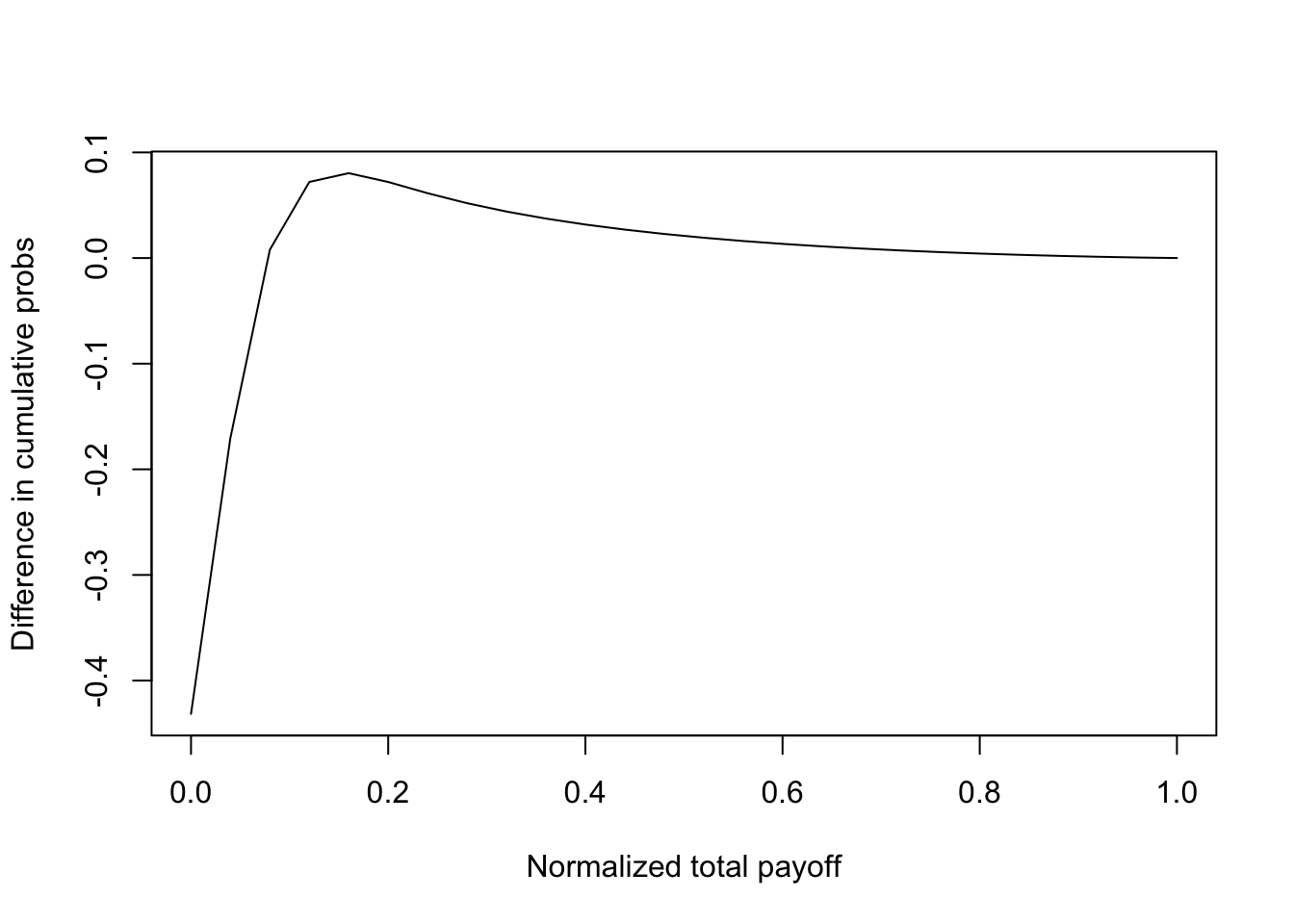
#CHECK IF SSD IS SATISFIED
#A SSD> B, if E(A)=E(B), and integral_0^y (F_A(z)-F_B(z)) dz <= 0, for all y
cumprobs2 = matrix(cumprobs2,length(cumprobs2),1)
n = length(cumprobs1)
ssd = NULL
for (j in 1:n) {
    check = sum(cumprobs1[1:j]-cumprobs2[1:j])
    ssd = c(ssd,check)
}
print(c("Max ssd = ",max(ssd)))  #If <0, then SSD satisfied, and it implies MV efficiency.
## [1] "Max ssd = " "-0.000556175706150297"plot(rets,ssd,type="l",xlab="Normalized total payoff",ylab="Integrated F(G[rho=0.09]) minus F(G[rho=0.81])")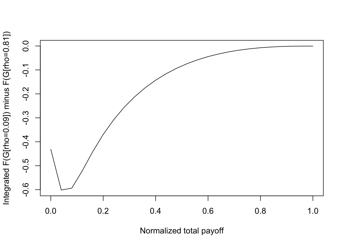
We look at expected utility.
#CHECK WHAT HAPPENS WITH UNEVEN WEIGHTS
#Result: No ordering with SSD, Utility lower if weights ascending.
#source("uneven_weights.R")
#Flat vs rising weights

num_names = 25
each_loss1 = array(13,num_names)
each_loss2 = seq(num_names)
each_prob = 0.05
rho = 0.55
gam = 3

for (j in seq(2)) {
    if (j==1) { L = each_loss1 }
    if (j==2) { L = each_loss2 }
    q = array(each_prob,num_names)
    res = digiprob(L,q,rho)
    rets = res[,1]/sum(each_loss1)
    probs = res[,2]
    cumprobs = array(0,length(res[,2]))
    cumprobs[1] = probs[1]
    for (k in seq(2,length(res[,2]))) {
        cumprobs[k] = cumprobs[k-1] + probs[k]
    }
    if (j==1) {
        plot(rets,cumprobs,type="l",xlab="Normalized Total Payoff",ylab="Cumulative Probability")
        cumprobs1 = cumprobs
        utility = sum(((0.1+rets)^(1-gam)/(1-gam))*probs)
    }
    if (j==2) {
        lines(rets,cumprobs,type="l",col="Red")
        cumprobs2 = cumprobs
        utility = sum(((0.1+rets)^(1-gam)/(1-gam))*probs)
    }
    mn = sum(rets*probs)
    idx = which(rets>0.01); p01 = sum(probs[idx])
    idx = which(rets>0.02); p02 = sum(probs[idx])
    idx = which(rets>0.03); p03 = sum(probs[idx])
    idx = which(rets>0.07); p07 = sum(probs[idx])
    idx = which(rets>0.10); p10 = sum(probs[idx])
    idx = which(rets>0.15); p15 = sum(probs[idx])
    idx = which(rets>0.25); p25 = sum(probs[idx])
    print(c(mn,p01,p02,p03,p07,p10,p15,p25))
    print(c("Utility = ",utility))
}
## [1] 0.04998222 0.49021241 0.49021241 0.49021241 0.27775760 0.16903478
## [7] 0.10711351 0.03051047
## [1] "Utility = "        "-33.7820026132803"
## [1] 0.04998222 0.46435542 0.43702188 0.40774167 0.25741601 0.17644497
## [7] 0.10250256 0.03688191
## [1] "Utility = "        "-34.4937532559838"
We now look at stochastic dominance.
#PLOT DIFFERENCE IN DISTRIBUTION FUNCTIONS
#IF POSITIVE FLAT WEIGHTS BETTER THAN RISING WEIGHTS
plot(rets,cumprobs1-cumprobs2,type="l",xlab="Normalized total payoff",ylab="Difference in cumulative probs")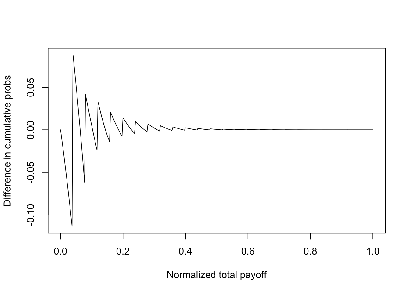
#CHECK IF SSD IS SATISFIED
#A SSD> B, if E(A)=E(B), and integral_0^y (F_A(z)-F_B(z)) dz <= 0, for all y
cumprobs2 = matrix(cumprobs2,length(cumprobs2),1)
n = length(cumprobs1)
ssd = NULL
for (j in 1:n) {
    check = sum(cumprobs1[1:j]-cumprobs2[1:j])
    ssd = c(ssd,check)
}
print(c("Max ssd = ",max(ssd)))  #If <0, then SSD satisfied, and it implies MV efficiency.
## [1] "Max ssd = " "0"19.10 Mixing safe and risky assets
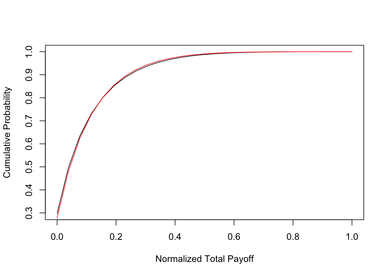
Is it better to have assets with a wide variation in probability of success or with similar probabilities? To examine this, we look at two portfolios of \(n=26\) assets. In the first portfolio, all the assets have a probability of success equal to \(q_i = 0.10\). In the second portfolio, half the firms have a success probability of \(0.05\) and the other half have a probability of \(0.15\). The payoff of all investments is \(1/26\). The probability distribution of payoffs and the expected utility for the same power utility investor (with \(\gamma=3\)) are given in code output below. We see that mixing the portfolio between investments with high and low probability of success results in higher expected utility than keeping the investments similar. We also confirmed that such imbalanced success probability portfolios also evidence SSD over portfolios with similar investments in terms of success rates. This result does not have a natural analog in the mean-variance world with non-digital assets. For empirical evidence on the efficacy of various diversification approaches, see (“The Performance of Private Equity Funds: Does Diversification Matter?” 2006).
#CHECK WHAT HAPPENS WITH MIXED PDs
#Result: No SSD ordering, but Utility higher for mixed pds
#source("mixed_pds.R")
num_names = 26
each_loss = array(1,num_names)
each_prob1 = array(0.10,num_names)
each_prob2 = c(array(0.05,num_names/2),array(0.15,num_names/2))
rho = 0.55
gam = 3 #Risk aversion CARA

for (j in seq(2)) {
    if (j==1) { q = each_prob1 }
    if (j==2) { q = each_prob2 }
    L = each_loss
    res = digiprob(L,q,rho)
    rets = res[,1]/sum(each_loss)
    probs = res[,2]
    cumprobs = array(0,length(res[,2]))
    cumprobs[1] = probs[1]
    for (k in seq(2,length(res[,2]))) {
        cumprobs[k] = cumprobs[k-1] + probs[k]
    }
    if (j==1) {
        plot(rets,cumprobs,type="l",xlab="Normalized Total Payoff",ylab="Cumulative Probability")
        cumprobs1 = cumprobs
        utility = sum(((0.1+rets)^(1-gam)/(1-gam))*probs)
    }
    if (j==2) {
        lines(rets,cumprobs,type="l",col="Red")
        cumprobs2 = cumprobs
        utility = sum(((0.1+rets)^(1-gam)/(1-gam))*probs)
    }
    mn = sum(rets*probs)
    idx = which(rets>0.01); p01 = sum(probs[idx])
    idx = which(rets>0.02); p02 = sum(probs[idx])
    idx = which(rets>0.03); p03 = sum(probs[idx])
    idx = which(rets>0.07); p07 = sum(probs[idx])
    idx = which(rets>0.10); p10 = sum(probs[idx])
    idx = which(rets>0.15); p15 = sum(probs[idx])
    idx = which(rets>0.25); p25 = sum(probs[idx])
    print(c(mn,p01,p02,p03,p07,p10,p15,p25))
    print(c("Utility = ",utility))
}
## [1] 0.09998225 0.70142788 0.70142788 0.70142788 0.50249327 0.36635887
## [7] 0.27007883 0.11105329
## [1] "Utility = "        "-24.6254789193705"
## [1] 0.09998296 0.72144189 0.72144189 0.72144189 0.51895166 0.37579336
## [7] 0.27345532 0.10589547
## [1] "Utility = "        "-23.9454295328498"
And of course, an examination of stochastic dominance.
#PLOT DIFFERENCE IN DISTRIBUTION FUNCTIONS
#IF POSITIVE EVERYWHERE MIXED PDs BETTER THAN FLAT PDs
plot(rets,cumprobs1-cumprobs2,type="l",xlab="Normalized total payoff",ylab="Difference in cumulative probs")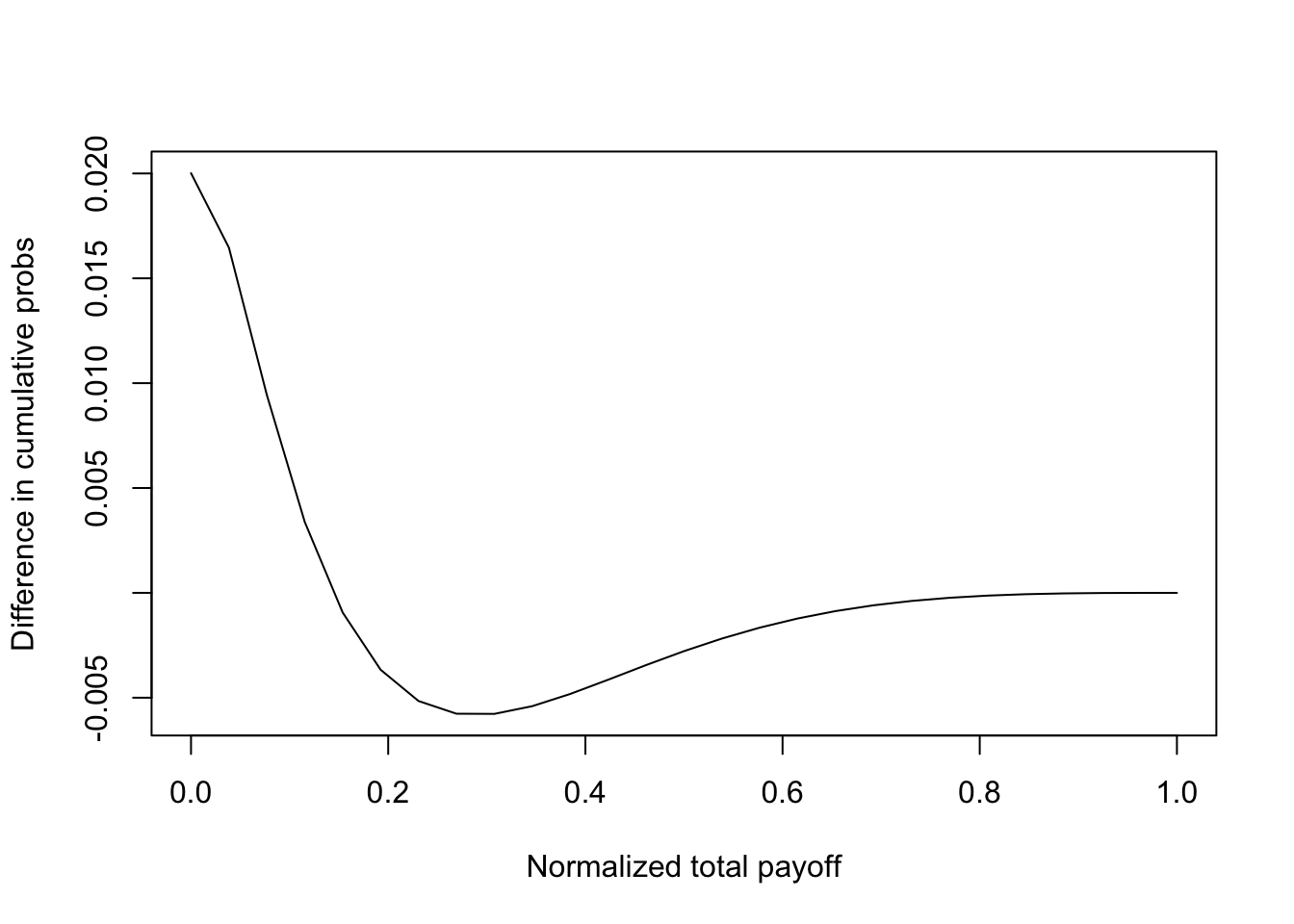
#CHECK IF SSD IS SATISFIED
#A SSD> B, if E(A)=E(B), and integral_0^y (F_A(z)-F_B(z)) dz <= 0, for all y
cumprobs2 = matrix(cumprobs2,length(cumprobs2),1)
n = length(cumprobs1)
ssd = NULL
for (j in 1:n) {
    check = sum(cumprobs2[1:j]-cumprobs1[1:j])
    ssd = c(ssd,check)
}
print(c("Max ssd = ",max(ssd)))  #If <0, then SSD satisfied, and it implies MV efficiency.
## [1] "Max ssd = " "-1.85123605385695e-05"19.11 Conclusions
Digital asset portfolios are different from mean-variance ones because the asset returns are Bernoulli with small success probabilities. We used a recursion technique borrowed from the credit portfolio literature to construct the payoff distributions for Bernoulli portfolios. We find that many intuitions for these portfolios are similar to those of mean-variance ones: diversification by adding assets is useful, low correlations amongst investments is good. However, we also find that uniform bet size is preferred to some small and some large bets. Rather than construct portfolios with assets having uniform success probabilities, it is preferable to have some assets with low success rates and others with high success probabilities, a feature that is noticed in the case of venture funds. These insights augment the standard understanding obtained from mean-variance portfolio optimization.
The approach taken here is simple to use. The only inputs needed are the expected payoffs of the assets \(C_i\), success probabilities \(q_i\), and the average correlation between assets, given by a parameter \(\rho\). Broad statistics on these inputs are available, say for venture investments, from papers such as Sarin, Das, and Jagannathan (2003). Therefore, using data, it is easy to optimize the portfolio of a digital asset fund. The technical approach here is also easily extended to features including cost of effort by investors as the number of projects grows (Kanniainen and Keuschnigg (2003)), syndication, etc. The number of portfolios with digital assets appears to be increasing in the marketplace, and the results of this analysis provide important intuition for asset managers.
The approach in Section 2 is just one way in which to model joint success probabilities using a common factor. Undeniably, there are other ways too, such as modeling joint probabilities directly, making sure that they are consistent with each other, which itself may be mathematically tricky. It is indeed possible to envisage that, for some different system of joint success probabilities, the qualitative nature of the results may differ from the ones developed here. It is also possible that the system we adopt here with a single common factor \(X\) may be extended to more than one common factor, an approach often taken in the default literature.
References
Das, Sanjiv. 2013. “Digital Portfolios.” The Journal of Portfolio Management Winter: 41–48.
Sarin, Atulya, Sanjiv Ranjan Das, and Murali Jagannathan. 2003. “The Private Equity Discount: An Empirical Examination of the Exit of Venture Backed Companies.” Journal of Investment Management 1 (1): 152–77.
Andersen, Leif, Jakob Sidenius, and Susanta Basu. 2003. “All Your Hedges in One Basket.” Risk November: 67–72.
“The Performance of Private Equity Funds: Does Diversification Matter?” 2006. Discussion Papers 192, SFB/TR 15, University of Munich.
Kanniainen, Vesa, and Christian Keuschnigg. 2003. “The Optimal Portfolio of Start-up Firms in Asset Capital Finance.” Journal of Corporate Finance 9 (5): 521–34.