Chapter 18 Being Mean with Variance: Markowitz Optimization
18.1 Diversification of a portfolio
It is useful to examine the power of using vector algebra with an application. Here we use vector and summation math to understand how diversification in stock portfolios works. Diversification occurs when we increase the number of non-perfectly correlated stocks in a portfolio, thereby reducing portfolio variance. In order to compute the variance of the portfolio we need to use the portfolio weights \({\bf w}\) and the covariance matrix of stock returns \({\bf R}\), denoted \({\bf \Sigma}\). We first write down the formula for a portfolio’s return variance:
\[ Var(\boldsymbol{w'R}) = \boldsymbol{w'\Sigma w} = \sum_{i=1}^n \boldsymbol{w_i^2 \sigma_i^2} + \sum_{i=1}^n \sum_{j=1,i \neq j}^n \boldsymbol{w_i w_j \sigma_{ij}} \]
Readers are strongly encouraged to implement this by hand for \(n=2\) to convince themselves that the vector form of the expression for variance \(\boldsymbol{w'\Sigma w}\) is the same thing as the long form on the right-hand side of the equation above. If returns are independent, then the formula collapses to:
\[ Var(\bf{w'R}) = \bf{w'\Sigma w} = \sum_{i=1}^n \boldsymbol{w_i^2 \sigma_i^2} \]
If returns are dependent, and equal amounts are invested in each asset (\(w_i=1/n,\;\;\forall i\)):
\[ \begin{align} Var(\bf{w'R}) &= \frac{1}{n}\sum_{i=1}^n \frac{\sigma_i^2}{n} + \frac{n-1}{n}\sum_{i=1}^n \sum_{j=1,i \neq j}^n \frac{\sigma_{ij}}{n(n-1)}\\ &= \frac{1}{n} \bar{\sigma_i}^2 + \frac{n-1}{n} \bar{\sigma_{ij}}\\ &= \frac{1}{n} \bar{\sigma_i}^2 + \left(1 - \frac{1}{n} \right) \bar{\sigma_{ij}} \end{align} \]
The first term is the average variance, denoted \(\bar{\sigma_1}^2\) divided by \(n\), and the second is the average covariance, denoted \(\bar{\sigma_{ij}}\) multiplied by factor \((n-1)/n\). As \(n \rightarrow \infty\),
\[ Var({\bf w'R}) = \bar{\sigma_{ij}} \]
This produces the remarkable result that in a well diversified portfolio, the variances of each stock’s return does not matter at all for portfolio risk! Further the risk of the portfolio, i.e., its variance, is nothing but the average of off-diagonal terms in the covariance matrix.
sd=0.50; cv=0.05; m=100
sd_p = matrix(0,m,1)
for (j in 1:m) {
    cv_mat = matrix(1,j,j)*cv
    diag(cv_mat) = sd^2
    w = matrix(1/j,j,1)
    sd_p[j] = sqrt(t(w) %*% cv_mat %*% w)
}

plot(sd_p,type="l",col="blue")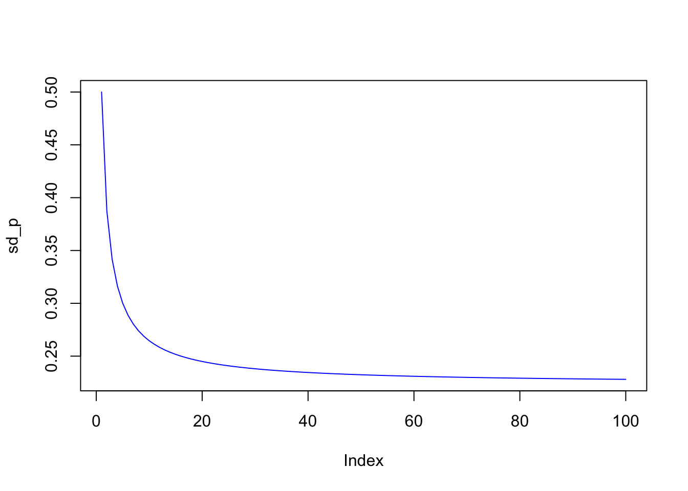
18.2 Markowitz Portfolio Problem
We now explore the mathematics of a famous portfolio optimization result, known as the Markowitz mean-variance problem. The solution to this problem is still being used widely in practice. We are interested in portfolios of \(n\) assets, which have a mean return which we denote as \(E(r_p)\), and a variance, denoted \(Var(r_p)\).
Let \(\underline{w} \in R^n\) be the portfolio weights. What this means is that we allocate each $1 into various assets, such that the total of the weights sums up to 1. Note that we do not preclude short-selling, so that it is possible for weights to be negative as well.
The optimization problem is defined as follows. We wish to find the portfolio that delivers the minimum variance (risk) while achieving a pre-specified level of expected (mean) return. \[ \min_{\underline{w}} \quad \frac{1}{2}\: \underline{w}' \underline{\Sigma} \: \underline{w} \] subject to \[ \begin{align} \underline{w}'\:\underline{\mu} &= E(r_p) \\ \underline{w}'\:\underline{1} &= 1 \end{align} \] Note that we have a \(\frac{1}{2}\) in front of the variance term above, which is for mathematical neatness as will become clear shortly. The minimized solution is not affected by scaling the objective function by a constant.
The first constraint forces the expected return of the portfolio to a specified mean return, denoted \(E(r_p)\), and the second constraint requires that the portfolio weights add up to 1, also known as the “fully invested” constraint. It is convenient that the constraints are equality constraints.
18.3 The Solution by Lagrange Multipliers
This is a Lagrangian problem, and requires that we embed the constraints into the objective function using Lagragian multipliers \(\{\lambda_1, \lambda_2\}\). This results in the following minimization problem:
\[ \min_{\underline{w}\, ,\lambda_1, \lambda_2} \quad L=\frac{1}{2}\:\underline{w}'\underline{\Sigma} \:\underline{w}+ \lambda_1[E(r_p)-\underline{w}'\underline{\mu}]+\lambda_2[1-\underline{w}'\underline{1}\;] \]
18.4 Optimization
To minimize this function, we take derivatives with respect to \(\underline{w}\), \(\lambda_1\), and \(\lambda_2\), to arrive at the first order conditions: \[ \begin{align} \frac{\partial L}{\partial \underline{w}} &= \underline{\Sigma}\underline{w} - \lambda_1 \underline{\mu} - \lambda_2 \underline{1}= \underline{0} \qquad(1) \\ \\ \frac{\partial L}{\partial \lambda_1} &= E(r_p)-\underline{w}'\underline{\mu}= 0 \\ \\ \frac{\partial L}{\partial \lambda_2} &= 1-\underline{w}'\underline{1}= 0 \end{align} \]
The first equation above, is a system of \(n\) equations, because the derivative is taken with respect to every element of the vector \(\underline{w}\). Hence, we have a total of \((n+2)\) first-order conditions. From (1)
\[ \begin{align} \underline{w} &= \Sigma^{-1}(\lambda_1\underline{\mu}+\lambda_2\underline{1}) \\ &= \lambda_1\Sigma^{-1}\underline{\mu}+\lambda_2\Sigma^{-1}\underline{1} \quad(2) \end{align} \]
Premultiply (2) by \(\underline{\mu}'\):
\[ \underline{\mu}'\underline{w}=\lambda_1\underbrace{\,\underline{\mu}'\underline{\Sigma}^{-1}\underline{\mu}\,}_B+ \lambda_2\underbrace{\,\underline{\mu}'\underline{\Sigma}^{-1}\underline{1}\,}_A=E(r_p) \]
Also premultiply (2) by \(\underline{1}'\):
\[\ \underline{1}'\underline{w}=\lambda_1\underbrace{\,\underline{1}'\underline{\Sigma}^{-1}\underline{\mu}}_A+ \lambda_2\underbrace{\,\underline{1}'\underline{\Sigma}^{-1}\underline{1}}_C=1 \]
Solve for \(\lambda_1, \lambda_2\) \[ \lambda_1=\frac{CE(r_p)-A}{D} \]
\[ \lambda_2=\frac{B-AE(r_p)}{D} \]
\[ \mbox{where} \quad D=BC-A^2 \]
18.5 Notes on the solution
Note 1: Since \(\underline{\Sigma}\) is positive definite, \(\underline{\Sigma}^{-1}\) is also positive definite: \(B>0, C>0\).
Note 2: Given solutions for \(\lambda_1, \lambda_2\), we solve for \(\underline{w}\).
\[ \underline{w}=\underbrace{\;\frac{1}{D}\,[B\underline{\Sigma}^{-1}\underline{1} -A\underline{\Sigma}^{-1}\underline{\mu}]}_{\underline{g}}+\underbrace{\;\frac{1}{D }\,[C\underline{\Sigma}^{-1}\underline{\mu} - A\underline{\Sigma}^{-1}\underline{1}\,]}_{\underline{h}}\cdot E(r_p) \]
This is the expression for the optimal portfolio weights that minimize the variance for given expected return \(E(r_p)\). We see that the vectors \(\underline{g}\), \(\underline{h}\) are fixed once we are given the inputs to the problem, i.e., \(\underline{\mu}\) and \(\underline{\Sigma}\).
Note 3: We can vary \(E(r_p)\) to get a set of frontier (efficient or optimal) portfolios \(\underline{w}\).
\[ \underline{w}=\underline{g}+\underline{h}\,E(r_p) \]
\[ \begin{align} if \quad E(r_p)&= 0,\; \underline{w} = \underline{g} \\ if \quad E(r_p)&= 1,\; \underline{w} = \underline{g}+\underline{h} \end{align} \]
Note that
\[ \underline{w}=\underline{g}+\underline{h}\,E(r_p)=[1-E(r_p)]\,\underline{g}+E(r_p)[\,\underline{g}+\underline{h}\:] \]
Hence these 2 portfolios \(\underline{g}\), \(\underline{g} + \underline{h}\) “generate” the entire frontier.
18.6 The Function
We create a function to return the optimal portfolio weights. Here is the code for the function to do portfolio optimization:
markowitz = function(mu,cv,Er) {
    n = length(mu)
    wuns = matrix(1,n,1)
    A = t(wuns) %*% solve(cv) %*% mu
    B = t(mu) %*% solve(cv) %*% mu
    C = t(wuns) %*% solve(cv) %*% wuns
    D = B*C - A^2
    lam = (C*Er-A)/D
    gam = (B-A*Er)/D
    wts = lam[1]*(solve(cv) %*% mu) + gam[1]*(solve(cv) %*% wuns)
    g = (B[1]*(solve(cv) %*% wuns) - A[1]*(solve(cv) %*% mu))/D[1]
    h = (C[1]*(solve(cv) %*% mu) - A[1]*(solve(cv) %*% wuns))/D[1]
    wts = g + h*Er
}
18.7 Example
We can enter an example of a mean return vector and the covariance matrix of returns, and then call the function for a given expected return.
#PARAMETERS
mu = matrix(c(0.02,0.10,0.20),3,1)
n = length(mu)
cv = matrix(c(0.0001,0,0,0,0.04,0.02,0,0.02,0.16),n,n)

print(mu)
## [,1]
## [1,] 0.02
## [2,] 0.10
## [3,] 0.20print(round(cv,4))## [,1] [,2] [,3]
## [1,] 1e-04 0.00 0.00
## [2,] 0e+00 0.04 0.02
## [3,] 0e+00 0.02 0.16The output is the vector of optimal portfolio weights.
Er = 0.18

#SOLVE PORTFOLIO PROBLEM
wts = markowitz(mu,cv,Er)
print(wts)
## [,1]
## [1,] -0.3575931
## [2,] 0.8436676
## [3,] 0.5139255print(sum(wts))## [1] 1print(t(wts) %*% mu)## [,1]
## [1,] 0.18print(sqrt(t(wts) %*% cv %*% wts))## [,1]
## [1,] 0.296793218.8 A different expected return
If we change the expected return to 0.10, then we get a different set of portfolio weights.
Er = 0.10

#SOLVE PORTFOLIO PROBLEM
wts = markowitz(mu,cv,Er)
print(wts)
## [,1]
## [1,] 0.3209169
## [2,] 0.4223496
## [3,] 0.2567335print(t(wts) %*% mu)## [,1]
## [1,] 0.1print(sqrt(t(wts) %*% cv %*% wts))## [,1]
## [1,] 0.1484205Note that in the first example, to get a high expected return of 0.18, we needed to take some leverage, by shorting the low risk asset and going long the medium and high risk assets. When we dropped the expected return to 0.10, all weights are positive, i.e., we have a long-only portfolio.
18.9 Numerical Optimization with Constraints
The quadprog package is an optimizer that takes a quadratic objective function with linear constraints. Hence, it is exactly what is needed for the mean-variance portfolio problem we just considered. The advantage of this package is that we can also apply additional inequality constraints. For example, we may not wish to permit short-sales of any asset, and thereby we might bound all the weights to lie between zero and one.
The specification in the quadprog package of the problem set up is shown in the manual:
Description

This routine implements the dual method of Goldfarb and
Idnani (1982, 1983) for solving quadratic programming
problems of the form min(-d^T b + 1/2 b^T D b) with the
constraints A^T b >= b_0.
(note: b here is the weights vector in our problem)

Usage
solve.QP(Dmat, dvec, Amat, bvec, meq=0, factorized=FALSE)

Arguments
Dmat     matrix appearing in the quadratic function to be minimized.
dvec     vector appearing in the quadratic function to be minimized.
Amat     matrix defining the constraints under which we want
     to minimize the quadratic function.
bvec     vector holding the values of b_0 (defaults to zero).
meq  the first meq constraints are treated as equality
     constraints, all further as inequality constraints
     (defaults to 0).
factorized   logical flag: if TRUE, then we are passing R^(-1)
     (where D = R^T R) instead of the matrix D in the
     argument Dmat.
\end{lstlisting}
In our problem set up, with three securities, and no short sales, we will have the following Amat and bvec. The constraints will be modulated by {meq = 2}, which states that the first two constraints will be equality constraints, and the last three will be greater than equal to constraints. The constraints will be of the form \(A'w \geq b_0\), i.e.,
\[ \begin{align} w_1 \mu_1 + w_2 \mu_2 + w_3 \mu_3 &= E(r_p) \\ w_1 1 + w_2 1 + w_3 1 &= 1 \\ w_1 &\geq 0\\ w_2 &\geq 0\\ w_3 &\geq 0 \end{align} \]
The code for using the package is as follows. If we run this code we get the following result for expected return = 0.18, with short-selling allowed.
#SOLVING THE PROBLEM WITH THE "quadprog" PACKAGE
Er = 0.18

library(quadprog)
nss = 0         #Equals 1 if no short sales allowed
Bmat = matrix(0,n,n)    #No Short sales matrix
diag(Bmat) = 1
Amat = matrix(c(mu,1,1,1),n,2)
if (nss==1) { Amat = matrix(c(Amat,Bmat),n,2+n) }
dvec = matrix(0,n,1)
bvec = matrix(c(Er,1),2,1)
if (nss==1) { bvec = t(c(bvec,matrix(0,3,1))) }
sol = solve.QP(cv,dvec,Amat,bvec,meq=2)
print(sol$solution)
## [1] -0.3575931 0.8436676 0.5139255This is exactly what is obtained from the Markowitz solution. Hence, the model checks out. What if we restricted short-selling? Then we would get the following solution.
#SOLVING THE PROBLEM WITH THE "quadprog" PACKAGE
Er = 0.18

library(quadprog)
nss = 1         #Equals 1 if no short sales allowed
Bmat = matrix(0,n,n)    #No Short sales matrix
diag(Bmat) = 1
Amat = matrix(c(mu,1,1,1),n,2)
if (nss==1) { Amat = matrix(c(Amat,Bmat),n,2+n) }
dvec = matrix(0,n,1)
bvec = matrix(c(Er,1),2,1)
if (nss==1) { bvec = t(c(bvec,matrix(0,3,1))) }
sol = solve.QP(cv,dvec,Amat,bvec,meq=2)
print(sol$solution)
## [1] 0.0 0.2 0.8wstar = as.matrix(sol$solution)
print(t(wstar) %*% mu)## [,1]
## [1,] 0.18print(sqrt(t(wstar) %*% cv %*% wstar))## [,1]
## [1,] 0.33226518.10 The Efficient Frontier
Since we can use the Markowitz model to solve for the optimal portfolio weights when the expected return is fixed, we can keep solving for different values of \(E(r_p)\). This will trace out the efficient frontier. The program to do this and plot the frontier is as follows.
#TRACING OUT THE EFFICIENT FRONTIER
Er_vec = as.matrix(seq(0.01,0.5,0.01))
Sig_vec = matrix(0,50,1)
j = 0
for (Er in Er_vec) {
    j = j+1
    wts = markowitz(mu,cv,Er)
    Sig_vec[j] = sqrt(t(wts) %*% cv %*% wts)
}
plot(Sig_vec,Er_vec,type='l')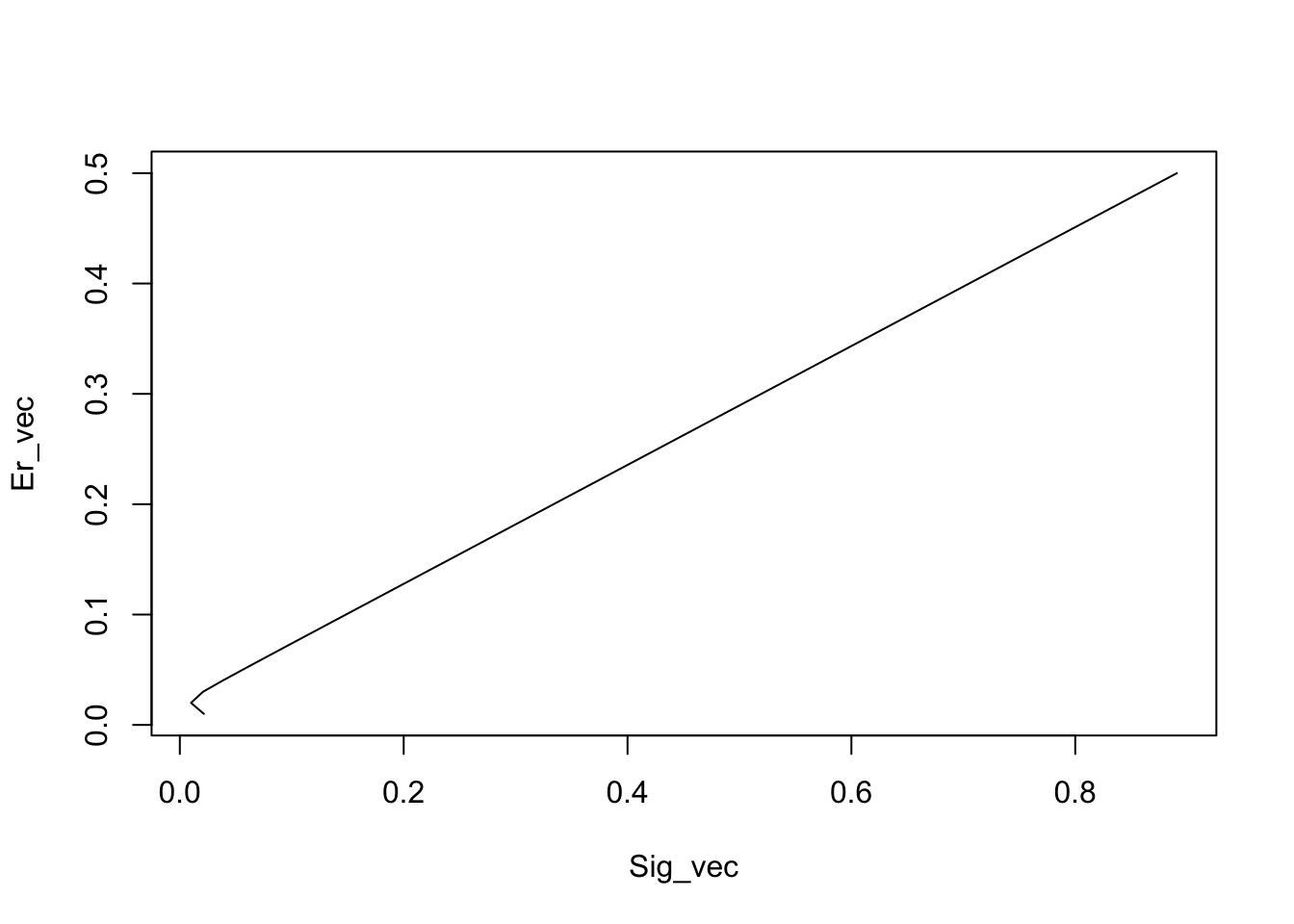
print(cbind(Sig_vec,Er_vec))## [,1] [,2]
## [1,] 0.021486319 0.01
## [2,] 0.009997134 0.02
## [3,] 0.020681789 0.03
## [4,] 0.038013721 0.04
## [5,] 0.056141450 0.05
## [6,] 0.074486206 0.06
## [7,] 0.092919536 0.07
## [8,] 0.111397479 0.08
## [9,] 0.129900998 0.09
## [10,] 0.148420529 0.10
## [11,] 0.166950742 0.11
## [12,] 0.185488436 0.12
## [13,] 0.204031572 0.13
## [14,] 0.222578791 0.14
## [15,] 0.241129149 0.15
## [16,] 0.259681974 0.16
## [17,] 0.278236773 0.17
## [18,] 0.296793176 0.18
## [19,] 0.315350898 0.19
## [20,] 0.333909721 0.20
## [21,] 0.352469471 0.21
## [22,] 0.371030008 0.22
## [23,] 0.389591219 0.23
## [24,] 0.408153014 0.24
## [25,] 0.426715315 0.25
## [26,] 0.445278059 0.26
## [27,] 0.463841194 0.27
## [28,] 0.482404674 0.28
## [29,] 0.500968460 0.29
## [30,] 0.519532521 0.30
## [31,] 0.538096827 0.31
## [32,] 0.556661353 0.32
## [33,] 0.575226080 0.33
## [34,] 0.593790987 0.34
## [35,] 0.612356059 0.35
## [36,] 0.630921280 0.36
## [37,] 0.649486639 0.37
## [38,] 0.668052123 0.38
## [39,] 0.686617722 0.39
## [40,] 0.705183428 0.40
## [41,] 0.723749232 0.41
## [42,] 0.742315127 0.42
## [43,] 0.760881106 0.43
## [44,] 0.779447163 0.44
## [45,] 0.798013292 0.45
## [46,] 0.816579490 0.46
## [47,] 0.835145750 0.47
## [48,] 0.853712070 0.48
## [49,] 0.872278445 0.49
## [50,] 0.890844871 0.50We can also simulate to see how the efficient frontier appears as the outer envelope of candidate portfolios.
#SIMULATE THE EFFICIENT FRONTIER
n = 10000
w = matrix(rnorm(2*n),n,2)
w = cbind(w,1-rowSums(w))
Exp_ret = w %*% mu
Sd_ret = matrix(0,n,1)
for (j in 1:n) {
    wt = as.matrix(w[j,])
    Sd_ret[j] = sqrt(t(wt) %*% cv %*% wt)
}
plot(Sd_ret,Exp_ret,col="red")
lines(Sig_vec,Er_vec,col="blue",lwd=6)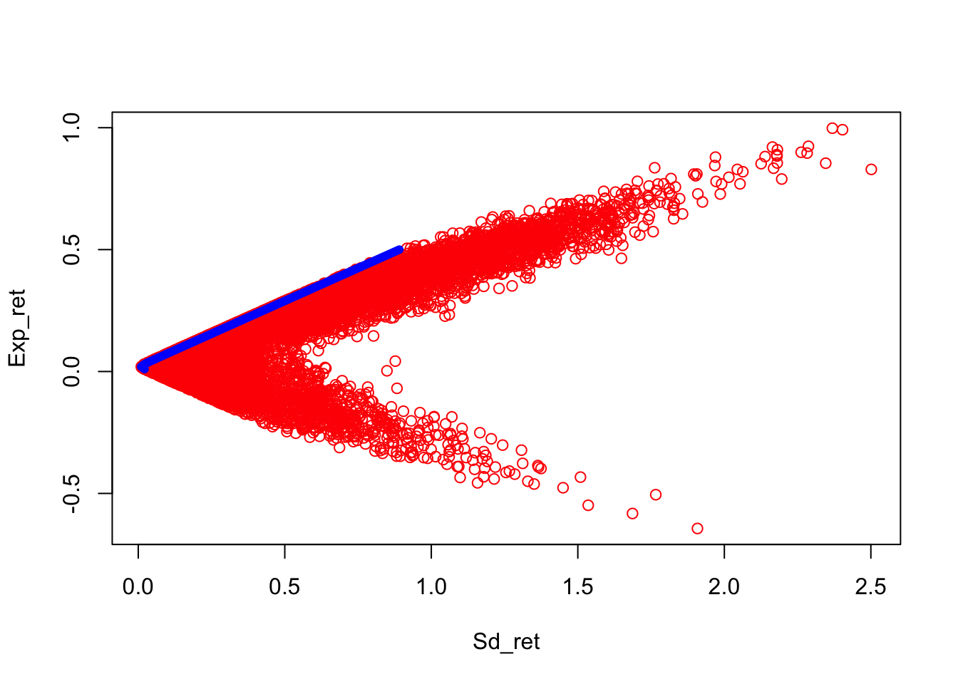
18.11 Covariances of frontier portfolios
Suppose we have two portfolios on the efficient frontier with weight vectors \(\underline{w}_p\) and \(\underline{w}_q\). The covariance between these two portfolios is:
\[ Cov(r_p,r_q)=\underline{w}_p'\:\underline{\Sigma}\:\underline{w}_q =[\underline{g}+\underline{h}E(r_p)]'\underline{\Sigma}\,[\underline{g} +\underline{h}E(r_q)] \]
Now, \[ \underline{g}+\underline{h}E(r_p)=\frac{1}{D}[B\underline{\Sigma}^{-1}\underline{1} -A\underline{\Sigma}^{-1}\underline{\mu}]+\frac{1}{D}[C\underline{\Sigma}^{-1}\underline{\mu} -A\underline{\Sigma}^{-1}\underline{1}\,]\underbrace{[\lambda_1B+\lambda_2A]}_{\frac{CE(r_p)-A}{D/B}+\frac{B-AE(r_p)}{D/B}} \]
After much simplification: \[ \begin{align} Cov(r_p,r_q) &= \underline{w}_p'\:\underline{\Sigma}\:\underline{w}_q' \\ &= \frac{C}{D}\,[E(r_p)-A/C][E(r_q)-A/C]+\frac{1}{C}\\ \\ \sigma^2_p=Cov(r_p,r_p)&= \frac{C}{D}[E(r_p)-A/C]^2+\frac{1}{C} \end{align} \]
Therefore, \[ \;\frac{\sigma^2_p}{1/C}-\frac{[E(r_p)-A/C]^2}{D/C^2}=1 \]
which is the equation of a hyperbola in \(\: \sigma, E(r)\) space with center \((0, A/C)\), or
\[ \sigma^2_p=\frac{1}{D}[CE(r_p)^2-2AE(r_p)+B], \]
which is a parabola in \(E(r), \sigma\) space.
18.12 Combinations
It is easy to see that linear combinations of portfolios on the frontier will also lie on the frontier.
\[ \begin{align} \sum_{i=1}^m \alpha_i\,\underline{w}_i &= \sum_{i=1}^m \alpha_i[\,\underline{g}+\underline{h}\,E(r_i)]\\ &= \underline{g}+\underline{h}\sum_{i=1}^m \alpha_iE(r_i) \\ \sum_{i=1}^m \alpha_i &=1 \end{align} \]
18.12.1 Exercise
Carry out the following analyses:
- Use your R program to do the following. Set \(E(r_p)=0.10\) (i.e. return of 10%), and solve for the optimal portfolio weights for your 3 securities. Call this vector of weights \(w_1\). Next, set \(E(r_p)=0.20\) and again solve for the portfolios weights \(w_2\).
- Take a 50/50 combination of these two portfolios. What are the weights? What is the expected return?
- For the expected return in the previous part, resolve the mean-variance problem to get the new weights?
- Compare these weights in part 3 to the ones in part 2 above. Explain your result.
This is a special portfolio of interest, and we will soon see why. Find
\[ E(r_q), \;s.t. \; \; Cov(r_p,r_q)=0 \] Suppose it exists, then the solution is:
\[ E(r_q)=\frac{A}{C}-\frac{D/C^2}{E(r_p)-A/C}\:\equiv\:E(r_{ZC(p)}) \]
Since \(ZC(p)\) exists for all p, all frontier portfolios can be formed from \(p\) and \(ZC(p)\).
\[ \begin{align} Cov(r_p,r_q) &=\underline{w}_p'\:\underline{\Sigma}\:\underline{w}_q \\ &=\lambda_1\underline{\mu}'\underline{\Sigma}^{-1}\underline{\Sigma}\: \underline{w}_q +\lambda_2\underline{1}'\underline{\Sigma}^{-1}\underline{\Sigma} \: \underline{w}_q \\ &= \lambda_1\underline{\mu}'\underline{w}_q+\lambda_2\underline{1}'\underline{w}_q\\ &= \lambda_1E(r_q)+\lambda_2 \end{align} \]
Substitute in for \(\lambda_1, \lambda_2\) and rearrange to get
\[ E(r_q)=(1- \beta_{qp})E[r_{ZC(p)}]+\beta_{qp}E(r_p) \]
\[ \beta_{qp}=\frac{Cov(r_q,r_p)}{\sigma_p^2} \] Therefore, the return on a portfolio can be written in terms of a basic portfolio \(p\) and its zero covariance portfolio \(ZC(p)\). This suggests a regression relationship, i.e. \[ r_q = \beta_0 + \beta_1 r_{ZC(p)}+ \beta_2 r_p + \xi \] which is nothing but a factor model, i.e. with orthogonal factors.
18.13 Portfolio problem with riskless assets
We now enhance the portfolio problem to deal with risk less assets. The difference is that the fully-invested constraint is expanded to include the risk free asset. We require just a single equality constraint. The problem may be specified as follows. \[ \min_{\underline{w}} \quad \frac{1}{2}\: \underline{w}' \underline{\Sigma} \: \underline{w} \]
\[ s.t. \quad \underline{w}'\underline{\mu}+(1-\underline{w}'\underline{1}\,)\,r_f=E(r_p) \]
The Lagrangian specification of the problem is as follows.
\[ \min_{\underline{w},\lambda} \quad L = \frac{1}{2}\:\underline{w}'\underline{\Sigma} \: \underline{w}+\lambda[E(r_p)-\underline{w}'\underline{\mu}-(1-\underline{w}'\underline{1})r_f] \]
The first-order conditions for the problem are as follows. \[ \begin{align} \frac{\partial L}{\partial \underline{w}}&= \underline{\Sigma} \: \underline{w} - \lambda \underline{\mu}+\lambda\,\underline{1}\,r_f=\underline{0}\\ \frac{\partial L}{\partial \lambda}&= E(r_p)-\underline{w}'\underline{\mu}-(1-\underline{w}'\underline{1})\,r_f=0 \end{align} \]
Re-aranging, and solving for \(\underline{w}\) and \(\lambda\), we get the following manipulations, eventually leading to the desired solution. \[ \begin{align} \underline{\Sigma} \: \underline{w}&= \lambda(\underline{\mu}-\underline{1}\:r_f)\\ E(r_p)-r_f&= \underline{w}'(\underline{\mu}-\underline{1}\:r_f) \end{align} \]
Take the first equation and proceed as follows: \[ \begin{align} \underline{w}&= \lambda \underline{\Sigma}^{-1} (\underline{\mu}-\underline{1}\:r_f)\\ E(r_p)-r_f \equiv (\underline{\mu} - \underline{1} r_f)' \underline{w}&= \lambda (\underline{\mu} - \underline{1} r_f)' \underline{\Sigma}^{-1} (\underline{\mu}-\underline{1}\:r_f)\\ \end{align} \]
The first and third terms in the equation above then give that \[ \lambda = \frac{E(r_p)-r_f}{(\underline{\mu} - \underline{1} r_f)' \underline{\Sigma}^{-1} (\underline{\mu}-\underline{1}\:r_f)} \]
Substituting this back into the first foc results in the final solution. \[ \underline{w}=\underline{\Sigma}^{-1}(\underline{\mu}-\underline{1}\:r_f)\frac{E(r_p)-r_f}{H} \]
\[ \mbox{where} \quad H=(\underline{\mu}-r_f\underline{1}\:)'\underline{\Sigma}^{-1}(\underline{\mu}-r_f\underline{1}\:) \] ### Example
We create a function for the solution to this problem, and then run the model.
markowitz2 = function(mu,cv,Er,rf) {
    n = length(mu)
    wuns = matrix(1,n,1)
    x = as.matrix(mu - rf*wuns)
    H = t(x) %*% solve(cv) %*% x
    wts = (solve(cv) %*% x) * (Er-rf)/H[1]
}
We run the code here.
#PARAMETERS
mu = matrix(c(0.02,0.10,0.20),3,1)
n = length(mu)
cv = matrix(c(0.0001,0,0,0,0.04,0.02,0,0.02,0.16),n,n)
Er = 0.18
rf = 0.01

sol = markowitz2(mu,cv,Er,rf)
print("Wts in stocks")
## [1] "Wts in stocks"print(sol)## [,1]
## [1,] 12.6613704
## [2,] 0.2236842
## [3,] 0.1223932print("Wts in risk free asset")## [1] "Wts in risk free asset"print(1-sum(sol))## [1] -12.00745print("Exp return")## [1] "Exp return"print(rf + t(sol) %*% (mu-rf))## [,1]
## [1,] 0.18print("Std Dev of return")## [1] "Std Dev of return"print(sqrt(t(sol) %*% cv %*% sol))## [,1]
## [1,] 0.1467117