Chapter 12 In the Same Boat: Cluster Analysis and Prediction Trees
12.1 Overview
There are many aspects of data analysis that call for grouping individuals, firms, projects, etc. These fall under the rubric of what may be termed as classification analysis. Cluster analysis comprises a group of techniques that uses distance metrics to bunch data into categories.
There are two broad approaches to cluster analysis:
Agglomerative or Hierarchical or Bottom-up: In this case we begin with all entities in the analysis being given their own cluster, so that we start with \(n\) clusters. Then, entities are grouped into clusters based on a given distance metric between each pair of entities. In this way a hierarchy of clusters is built up and the researcher can choose which grouping is preferred.
Partitioning or Top-down: In this approach, the entire set of \(n\) entities is assumed to be a cluster. Then it is progressively partitioned into smaller and smaller clusters.
We will employ both clustering approaches and examine their properties with various data sets as examples.
12.2 k-MEANS
This approach is bottom-up. If we have a sample of \(n\) observations to be allocated to \(k\) clusters, then we can initialize the clusters in many ways. One approach is to assume that each observation is a cluster unto itself. We proceed by taking each observation and allocating it to the nearest cluster using a distance metric. At the outset, we would simply allocate an observation to its nearest neighbor.
How is nearness measured? We need a distance metric, and one common one is Euclidian distance. Suppose we have two observations \(x_i\) and \(x_j\). These may be represented by a vector of attributes. Suppose our observations are people, and the attributes are {height, weight, IQ} = \(x_i = \{h_i, w_i, I_i\}\) for the \(i\)-th individual. Then the Euclidian distance between two individuals \(i\) and \(j\) is
\[ d_{ij} = \sqrt{(h_i-h_j)^2 + (w_i-w_j)^2 + (I_i - I_j)^2} \]
It is usually computed using normalized variables, so that no single variable of large size dominates the distance calculation. (Normalization is the process of subtracting the mean from each observation and then dividing by the standard deviation.)
In contrast, the “Manhattan” distance is given by (when is this more appropriate?)
\[ d_{ij} = |h_i-h_j| + |w_i-w_j| + |I_i - I_j| \]
We may use other metrics such as the cosine distance, or the Mahalanobis distance. A matrix of \(n \times n\) values of all \(d_{ij}\)s is called the distance matrix. Using this distance metric we assign nodes to clusters or attach them to nearest neighbors. After a few iterations, no longer are clusters made up of singleton observations, and the number of clusters reaches \(k\), the preset number required, and then all nodes are assigned to one of these \(k\) clusters. As we examine each observation we then assign it (or re-assign it) to the nearest cluster, where the distance is measured from the observation to some representative node of the cluster. Some common choices of the representative node in a cluster of are:
- Centroid of the cluster. This is the mean of the observations in the cluster for each attribute. The centroid of the two observations above is the average vector \(\{(h_i+h_j)/2, (w_i+w_j)/2, (I_i + I_j)/2\}\). This is often called the center of the cluster. If there are more nodes then the centroid is the average of the same coordinate for all nodes.
- Closest member of the cluster.
- Furthest member of the cluster.
The algorithm converges when no re-assignments of observations to clusters occurs. Note that \(k\)-means is a random algorithm, and may not always return the same clusters every time the algorithm is run. Also, one needs to specify the number of clusters to begin with and there may be no a-priori way in which to ascertain the correct number. Hence, trial and error and examination of the results is called for. Also, the algorithm aims to have balanced clusters, but this may not always be appropriate.
In R, we may construct the distance matrix using the dist function. Using the NCAA data we are already familiar with, we have:
ncaa = read.table("DSTMAA_data/ncaa.txt",header=TRUE)
print(names(ncaa))
## [1] "No" "NAME" "GMS" "PTS" "REB" "AST" "TO" "A.T" "STL" "BLK"
## [11] "PF" "FG" "FT" "X3P"d = dist(ncaa[,3:14], method="euclidian")
print(head(d))## [1] 12.842301 10.354557 7.996641 9.588546 15.892854 20.036546Examining this matrix will show that it contains \(n(n-1)/2\) elements, i.e., the number of pairs of nodes. Only the lower triangular matrix of \(d\) is populated.
Clustering takes many observations with their characteristics and then allocates them into buckets or clusters based on their similarity. In finance, we may use cluster analysis to determine groups of similar firms.
Unlike regression analysis, cluster analysis uses only the right-hand side variables, and there is no dependent variable required. We group observations purely on their overall similarity across characteristics. Hence, it is closely linked to the notion of communities that we studied in network analysis, though that concept lives primarily in the domain of networks.
12.2.1 Example: Randomly generated data in k-means
Here we use the example from the kmeans function to see how the clusters appear. This function is standard issue, i.e., it comes with the stats package, which is included in the base R distribution and does not need to be separately installed. The data is randomly generated but has two bunches of items with different means, so we should be easily able to see two separate clusters. You will need the graphics package which is also in the base installation.
# a 2-dimensional example
x <- rbind(matrix(rnorm(100, sd = 0.3), ncol = 2),
           matrix(rnorm(100, mean = 1, sd = 0.3), ncol = 2))
colnames(x) <- c("x", "y")
(cl <- kmeans(x, 2))
## K-means clustering with 2 clusters of sizes 49, 51
##
## Cluster means:
## x y
## 1 1.04959200 1.05894643
## 2 -0.01334206 0.02180248
##
## Clustering vector:
## [1] 2 2 2 2 2 2 2 2 2 2 2 2 2 2 2 2 2 2 2 2 2 2 2 2 2 2 2 2 2 2 2 2 2 2 2
## [36] 2 2 2 2 2 2 2 2 2 2 2 2 2 2 2 2 1 1 1 1 1 1 1 1 1 1 1 1 1 1 1 1 1 1 1
## [71] 1 1 1 1 1 1 1 1 1 1 1 1 1 1 1 1 1 1 1 1 1 1 1 1 1 1 1 1 1 1
##
## Within cluster sum of squares by cluster:
## [1] 11.059361 9.740516
## (between_SS / total_SS = 72.6 %)
##
## Available components:
##
## [1] "cluster"      "centers"      "totss"        "withinss"
## [5] "tot.withinss" "betweenss"    "size"         "iter"
## [9] "ifault"#PLOTTING CLUSTERS
print(names(cl))## [1] "cluster" "centers" "totss" "withinss"
## [5] "tot.withinss" "betweenss" "size" "iter"
## [9] "ifault"plot(x, col = cl$cluster)
points(cl$centers, col = 1:2, pch = 8, cex=4)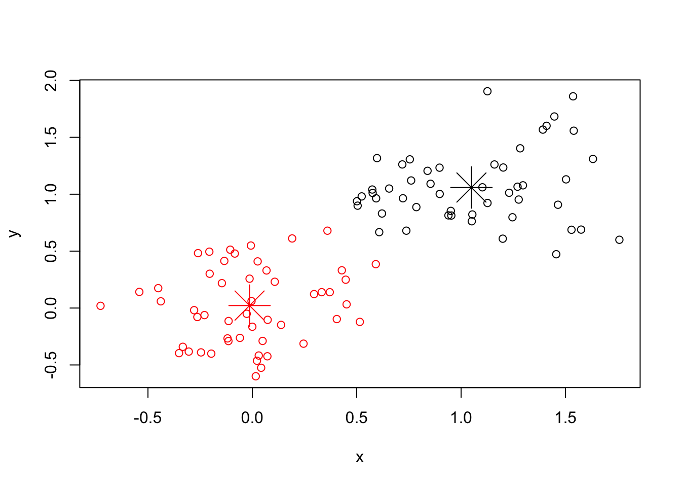
#REDO ANALYSIS WITH 5 CLUSTERS
## random starts do help here with too many clusters
(cl <- kmeans(x, 5, nstart = 25))
## K-means clustering with 5 clusters of sizes 24, 16, 23, 27, 10
##
## Cluster means:
## x y
## 1 0.1426836 0.3005998
## 2 1.3211293 0.8482919
## 3 0.7201982 0.9970443
## 4 -0.1520315 -0.2260174
## 5 1.3727382 1.5383686
##
## Clustering vector:
## [1] 1 1 1 4 4 1 4 1 4 4 4 4 1 1 4 1 1 1 4 4 4 1 1 4 4 1 1 4 4 1 4 4 4 4 4
## [36] 4 1 1 4 1 4 4 4 1 4 1 1 1 1 4 1 2 5 5 3 3 3 3 2 3 5 3 3 3 3 3 3 2 2 2
## [71] 5 2 2 3 2 3 5 2 2 3 5 2 5 5 3 3 3 3 3 3 3 2 3 3 2 2 5 2 2 5
##
## Within cluster sum of squares by cluster:
## [1] 2.6542258 1.2278786 1.2401518 2.4590282 0.7752739
## (between_SS / total_SS = 89.0 %)
##
## Available components:
##
## [1] "cluster" "centers" "totss" "withinss"
## [5] "tot.withinss" "betweenss" "size" "iter"
## [9] "ifault"plot(x, col = cl$cluster)
points(cl$centers, col = 1:5, pch = 8)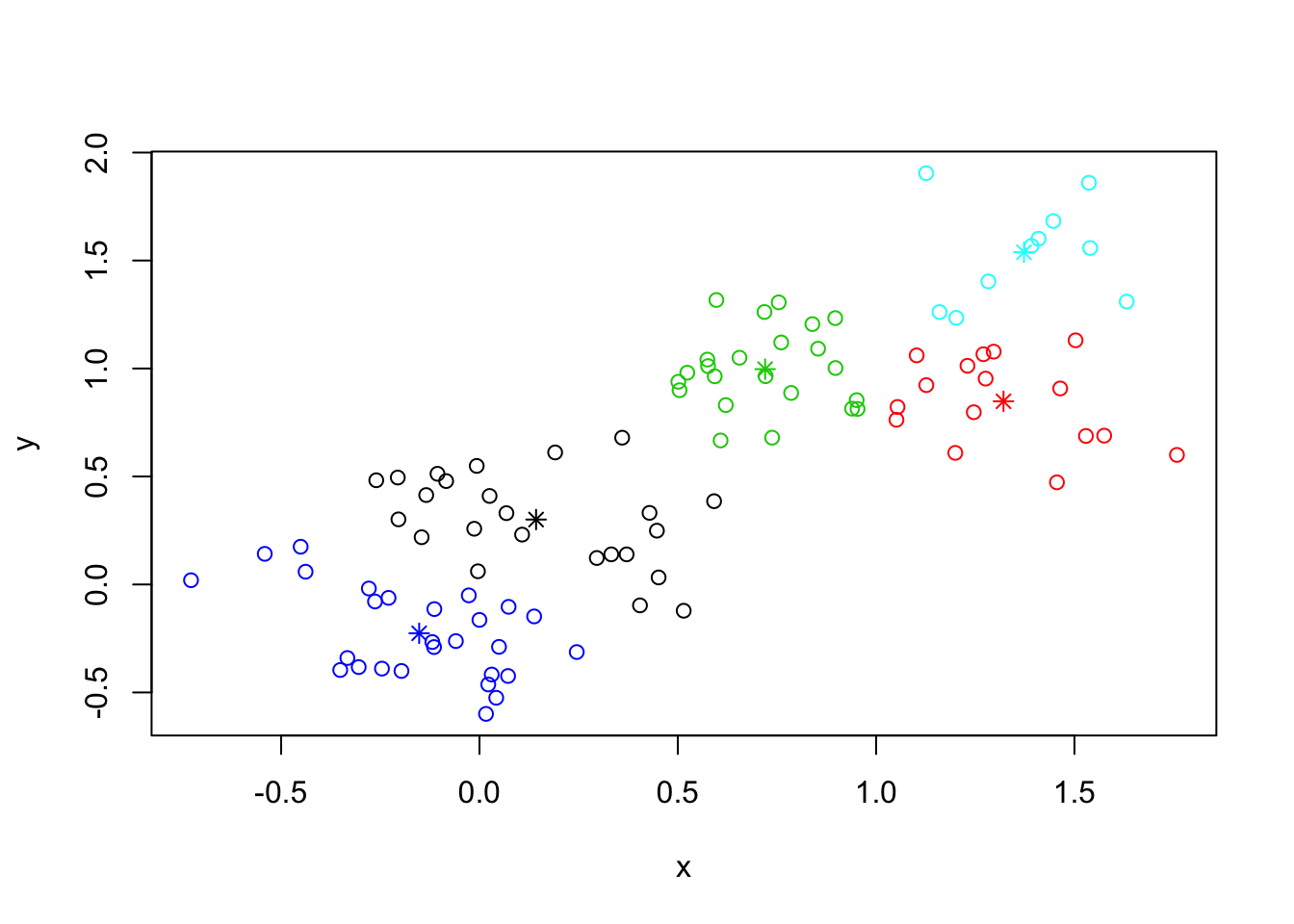
12.2.2 Example: NCAA teams
We revisit our NCAA data set, and form clusters there.
ncaa = read.table("DSTMAA_data/ncaa.txt",header=TRUE)
print(names(ncaa))
## [1] "No" "NAME" "GMS" "PTS" "REB" "AST" "TO" "A.T" "STL" "BLK"
## [11] "PF" "FG" "FT" "X3P"fit = kmeans(ncaa[,3:14],4)
print(fit$size)## [1] 6 27 14 17print(fit$centers)## GMS PTS REB AST TO A.T STL
## 1 1.000000 50.33333 28.83333 10.333333 12.50000 0.9000000 6.666667
## 2 1.777778 68.39259 33.17407 13.596296 12.83704 1.1107407 6.822222
## 3 3.357143 80.12857 34.15714 16.357143 13.70714 1.2357143 6.821429
## 4 1.529412 60.24118 38.76471 9.282353 16.45882 0.5817647 6.882353
## BLK PF FG FT X3P
## 1 2.166667 19.33333 0.3835000 0.6565000 0.2696667
## 2 2.918519 18.68519 0.4256296 0.7071852 0.3263704
## 3 2.514286 18.48571 0.4837143 0.7042143 0.4035714
## 4 2.882353 18.51176 0.3838824 0.6683529 0.3091765#Since there are more than two attributes of each observation in the data,
#we picked two of them {AST, PTS} and plotted the clusters against those.
idx = c(4,6)
plot(ncaa[,idx],col=fit$cluster)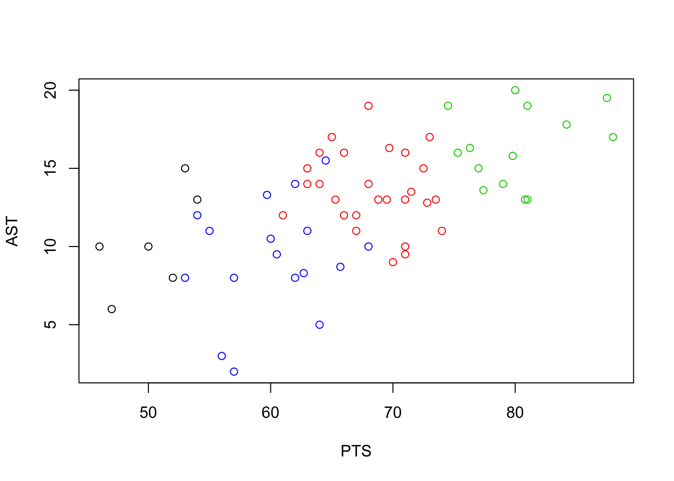
12.3 Hierarchical Clustering
Hierarchical clustering is both, a top-down (divisive) approach and bottom-up (agglomerative) approach. At the top level there is just one cluster. A level below, this may be broken down into a few clusters, which are then further broken down into more sub-clusters a level below, and so on. This clustering approach is computationally expensive, and the divisive approach is exponentially expensive in \(n\), the number of entities being clustered. In fact, the algorithm is \({\cal O}(2^n)\).
The function for clustering is hclust and is included in the stats package in the base R distribution.
We begin by first computing the distance matrix. Then we call the hclust function and the plot function applied to object fit gives what is known as a dendrogram plot, showing the cluster hierarchy. We may pick clusters at any level. In this case, we chose a cut level such that we get four clusters, and the rect.hclust function allows us to superimpose boxes on the clusters so we can see the grouping more clearly. The result is plotted in the Figure below.
d = dist(ncaa[,3:14], method="euclidian")
fit = hclust(d, method="ward")
## The "ward" method has been renamed to "ward.D"; note new "ward.D2"names(fit)## [1] "merge" "height" "order" "labels" "method"
## [6] "call" "dist.method"plot(fit,main="NCAA Teams")
groups = cutree(fit, k=3)
rect.hclust(fit, k=3, border="blue")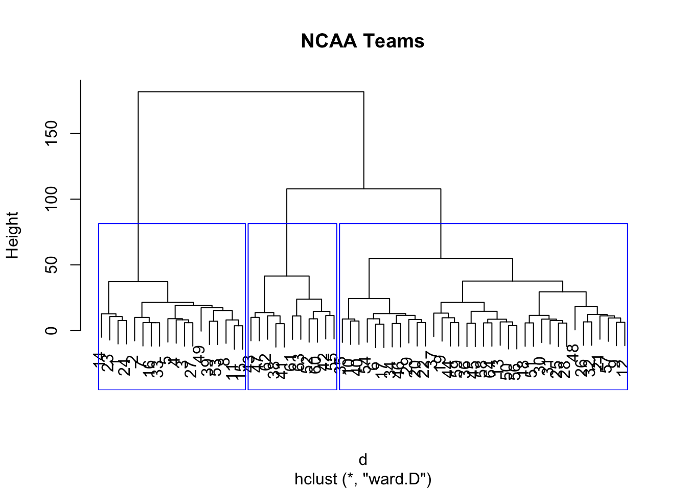
We can also visualize the clusters loaded on to the top two principal components as follows, using the clusplot function that resides in package cluster. The result is plotted in the Figure below.
print(groups)## [1] 1 1 1 1 1 2 1 1 2 2 1 2 2 1 1 1 2 2 2 2 2 2 1 1 2 2 1 2 2 2 2 2 1 2 2
## [36] 2 2 3 1 2 3 3 3 2 2 2 3 2 1 2 2 3 1 2 3 2 2 2 2 3 3 3 3 2library(cluster)
clusplot(ncaa[,3:14],groups,color=TRUE,shade=TRUE,labels=2,lines=0)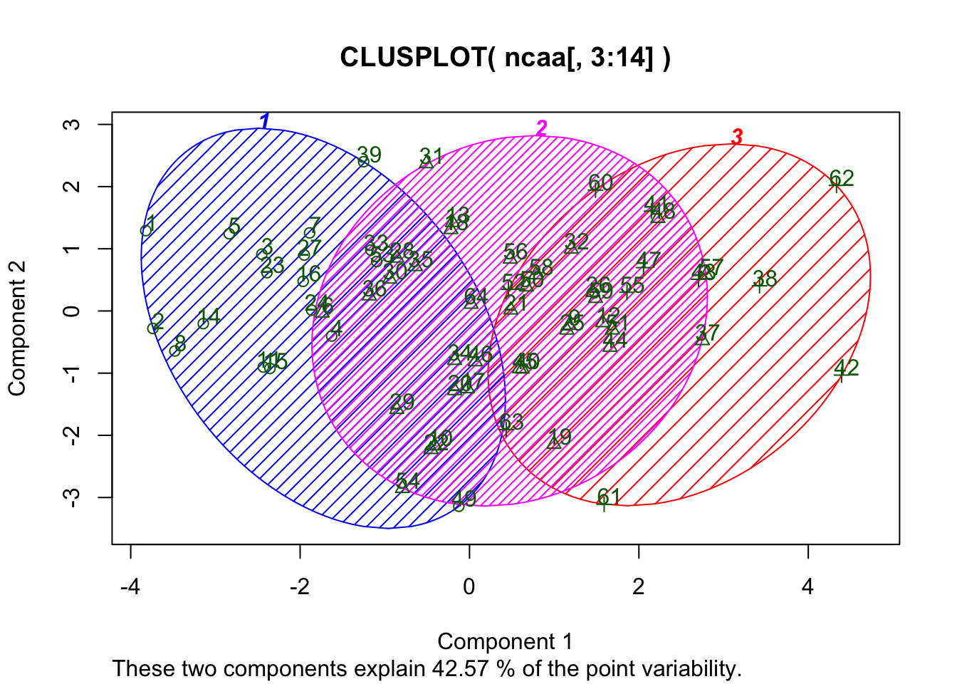
#Using the correlation matrix as a proxy for distance
x = t(as.matrix(ncaa[,3:14]))
d = as.dist((1-cor(x))/2)
fit = hclust(d, method="ward")
## The "ward" method has been renamed to "ward.D"; note new "ward.D2"plot(fit,main="NCAA Teams")
groups = cutree(fit, k=3)
rect.hclust(fit, k=3, border="red")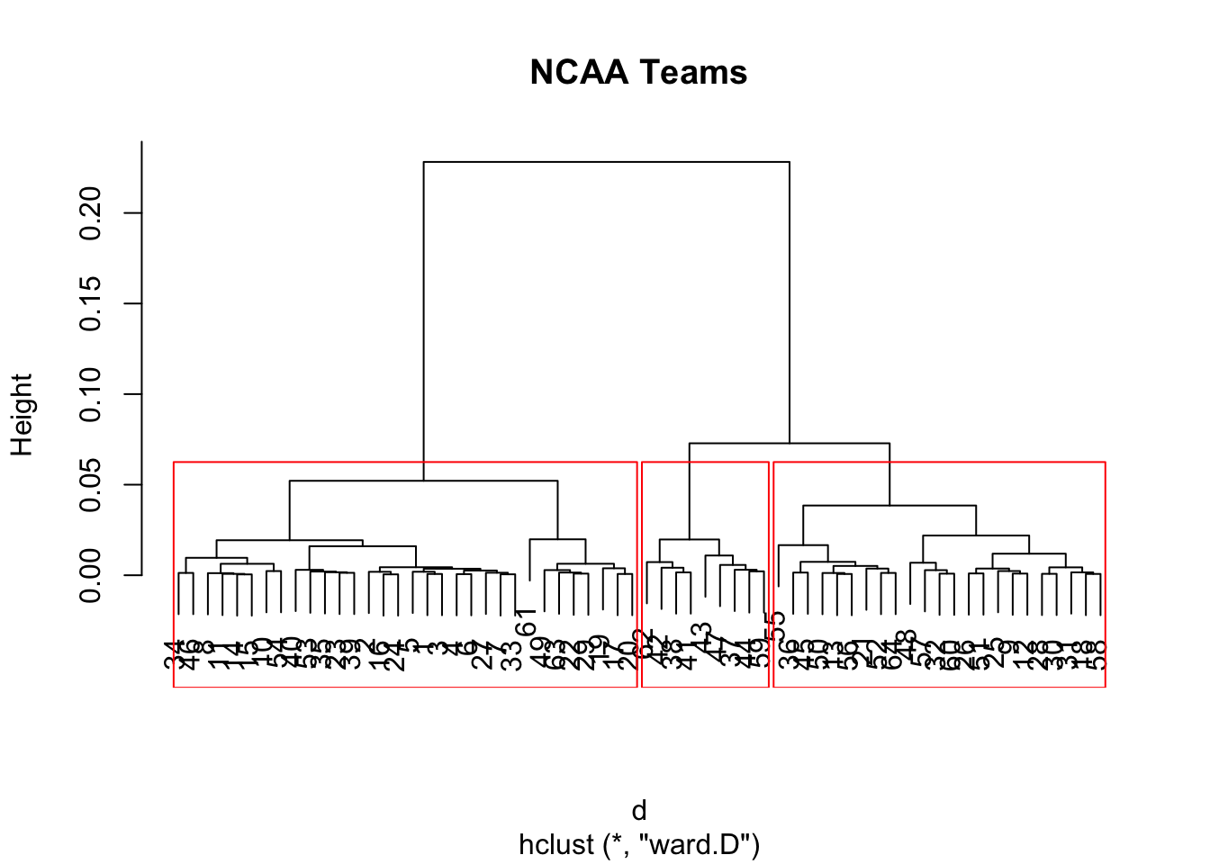
print(groups)## [1] 1 1 1 1 1 1 1 1 2 1 1 2 2 1 1 1 1 2 1 1 2 1 1 1 2 2 1 2 1 2 2 2 1 1 1
## [36] 2 3 3 1 1 3 3 3 3 2 1 3 2 1 2 2 2 1 1 2 2 2 2 3 2 1 3 1 2library(cluster)
clusplot(ncaa[,3:14],groups,color=TRUE,shade=TRUE,labels=2,lines=0)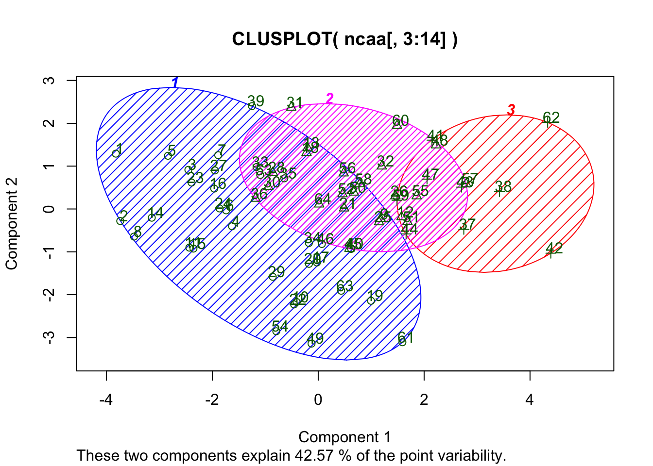
12.4 k Nearest Neighbors
This is one of the simplest algorithms for classification and grouping. Simply define a distance metric over a set of observations, each with \(M\) characteristics, i.e., \(x_1, x_2,..., x_M\). Compute the pairwise distance between each pair of observations, using any of the metrics above.
Next, fix \(k\), the number of nearest neighbors in the population to be considered. Finally, assign the category based on which one has the majority of nearest neighbors to the case we are trying to classify.
We see an example in R using the iris data set that we examined before.
library(class)
data(iris)
print(head(iris))
## Sepal.Length Sepal.Width Petal.Length Petal.Width Species
## 1 5.1 3.5 1.4 0.2 setosa
## 2 4.9 3.0 1.4 0.2 setosa
## 3 4.7 3.2 1.3 0.2 setosa
## 4 4.6 3.1 1.5 0.2 setosa
## 5 5.0 3.6 1.4 0.2 setosa
## 6 5.4 3.9 1.7 0.4 setosa#SAMPLE A SUBSET
idx = seq(1,length(iris[,1]))
train_idx = sample(idx,100)
test_idx = setdiff(idx,train_idx)
x_train = iris[train_idx,1:4]
x_test = iris[test_idx,1:4]
y_train = iris[train_idx,5]
y_test = iris[test_idx,5]
#RUN knn
res = knn(x_train, x_test, y_train, k = 3, prob = FALSE, use.all = TRUE)
res## [1] setosa setosa setosa setosa setosa setosa
## [7] setosa setosa setosa setosa setosa setosa
## [13] setosa setosa setosa versicolor versicolor versicolor
## [19] versicolor versicolor versicolor versicolor versicolor versicolor
## [25] versicolor versicolor versicolor versicolor versicolor versicolor
## [31] virginica versicolor versicolor versicolor versicolor virginica
## [37] virginica virginica virginica virginica virginica virginica
## [43] virginica virginica virginica virginica virginica virginica
## [49] virginica virginica
## Levels: setosa versicolor virginicatable(res,y_test)## y_test
## res setosa versicolor virginica
## setosa 15 0 0
## versicolor 0 19 0
## virginica 0 1 1512.5 Prediction Trees
Prediction trees are a natural outcome of recursive partitioning of the data. Hence, they are a particular form of clustering at different levels. Usual cluster analysis results in a flat partition, but prediction trees develop a multi-level cluster of trees. The term used here is CART, which stands for classification analysis and regression trees. But prediction trees are different from vanilla clustering in an important way – there is a dependent variable, i.e., a category or a range of values (e.g., a score) that one is attempting to predict.
Prediction trees are of two types: (a) Classification trees, where the leaves of the trees are different categories of discrete outcomes. and (b) Regression trees, where the leaves are continuous outcomes. We may think of the former as a generalized form of limited dependent variables, and the latter as a generalized form of regression analysis.
To set ideas, suppose we want to predict the credit score of an individual using age, income, and education as explanatory variables. Assume that income is the best explanatory variable of the three. Then, at the top of the tree, there will be income as the branching variable, i.e., if income is less than some threshold, then we go down the left branch of the tree, else we go down the right. At the next level, it may be that we use education to make the next bifurcation, and then at the third level we use age. A variable may even be repeatedly used at more than one level. This leads us to several leaves at the bottom of the tree that contain the average values of the credit scores that may be reached. For example if we get an individual of young age, low income, and no education, it is very likely that this path down the tree will lead to a low credit score on average. Instead of credit score (an example of a regression tree), consider credit ratings of companies (an example of a classification tree). These ideas will become clearer once we present some examples.
12.5.1 Fitting the tree
Recursive partitioning is the main algorithmic construct behind prediction trees. We take the data and using a single explanatory variable, we try and bifurcate the data into two categories such that the additional information from categorization results in better information than before the binary split. For example, suppose we are trying to predict who will make donations and who will not using a single variable – income. If we have a sample of people and have not yet analyzed their incomes, we only have the raw frequency \(p\) of how many people made donations, i.e., and number between 0 and 1. The information of the predicted likelihood \(p\) is inversely related to the sum of squared errors (SSE) between this value \(p\) and the 0 values and 1 values of the observations.
\[ SSE_1 = \sum_{i=1}^n (x_i - p)^2 \]
where \(x_i = \{0,1\}\), depending on whether person \(i\) made a donation or not. Now, if we bifurcate the sample based on income, say to the left we have people with income less than \(K\), and to the right, people with incomes greater than or equal to \(K\). If we find that the proportion of people on the left making donations is \(p_L < p\) and on the right is \(p_R > p\), our new information is:
\[ SSE_2 = \sum_{i, Income < K} (x_i - p_L)^2 + \sum_{i, Income \geq K} (x_i - p_R)^2 \]
By choosing \(K\) correctly, our recursive partitioning algorithm will maximize the gain, i.e., \(\delta = (SSE_1 - SSE_2)\). We stop branching further when at a given tree level \(\delta\) is less than a pre-specified threshold.
We note that as \(n\) gets large, the computation of binary splits on any variable is expensive, i.e., of order \({\cal O}(2^n)\). But as we go down the tree, and use smaller subsamples, the algorithm becomes faster and faster. In general, this is quite an efficient algorithm to implement.
The motivation of prediction trees is to emulate a decision tree. It also helps make sense of complicated regression scenarios where there are lots of variable interactions over many variables, when it becomes difficult to interpret the meaning and importance of explanatory variables in a prediction scenario. By proceeding in a hierarchical manner on a tree, the decision analysis becomes transparent, and can also be used in practical settings to make decisions.
12.6 Classification Trees
To demonstrate this, let’s use a data set that is already in R. We use the kyphosis data set which contains data on children who have had spinal surgery. The model we wish to fit is to predict whether a child has a post-operative deformity or not (variable: Kyphosis = {absent, present}). The variables we use are Age in months, number of vertebrae operated on (Number), and the beginning of the range of vertebrae operated on (Start). The package used is called rpart which stands for recursive partitioning.
library(rpart)
data(kyphosis)
head(kyphosis)
## Kyphosis Age Number Start
## 1 absent 71 3 5
## 2 absent 158 3 14
## 3 present 128 4 5
## 4 absent 2 5 1
## 5 absent 1 4 15
## 6 absent 1 2 16fit = rpart(Kyphosis~Age+Number+Start, method="class", data=kyphosis)
printcp(fit)##
## Classification tree:
## rpart(formula = Kyphosis ~ Age + Number + Start, data = kyphosis,
## method = "class")
##
## Variables actually used in tree construction:
## [1] Age Start
##
## Root node error: 17/81 = 0.20988
##
## n= 81
##
## CP nsplit rel error xerror xstd
## 1 0.176471 0 1.00000 1.0000 0.21559
## 2 0.019608 1 0.82353 1.2353 0.23200
## 3 0.010000 4 0.76471 1.2353 0.23200summary(kyphosis)## Kyphosis Age Number Start
## absent :64 Min. : 1.00 Min. : 2.000 Min. : 1.00
## present:17 1st Qu.: 26.00 1st Qu.: 3.000 1st Qu.: 9.00
## Median : 87.00 Median : 4.000 Median :13.00
## Mean : 83.65 Mean : 4.049 Mean :11.49
## 3rd Qu.:130.00 3rd Qu.: 5.000 3rd Qu.:16.00
## Max. :206.00 Max. :10.000 Max. :18.00summary(fit)## Call:
## rpart(formula = Kyphosis ~ Age + Number + Start, data = kyphosis,
## method = "class")
## n= 81
##
## CP nsplit rel error xerror xstd
## 1 0.17647059 0 1.0000000 1.000000 0.2155872
## 2 0.01960784 1 0.8235294 1.235294 0.2320031
## 3 0.01000000 4 0.7647059 1.235294 0.2320031
##
## Variable importance
## Start Age Number
## 64 24 12
##
## Node number 1: 81 observations, complexity param=0.1764706
## predicted class=absent expected loss=0.2098765 P(node) =1
## class counts: 64 17
## probabilities: 0.790 0.210
## left son=2 (62 obs) right son=3 (19 obs)
## Primary splits:
## Start < 8.5 to the right, improve=6.762330, (0 missing)
## Number < 5.5 to the left, improve=2.866795, (0 missing)
## Age < 39.5 to the left, improve=2.250212, (0 missing)
## Surrogate splits:
## Number < 6.5 to the left, agree=0.802, adj=0.158, (0 split)
##
## Node number 2: 62 observations, complexity param=0.01960784
## predicted class=absent expected loss=0.09677419 P(node) =0.7654321
## class counts: 56 6
## probabilities: 0.903 0.097
## left son=4 (29 obs) right son=5 (33 obs)
## Primary splits:
## Start < 14.5 to the right, improve=1.0205280, (0 missing)
## Age < 55 to the left, improve=0.6848635, (0 missing)
## Number < 4.5 to the left, improve=0.2975332, (0 missing)
## Surrogate splits:
## Number < 3.5 to the left, agree=0.645, adj=0.241, (0 split)
## Age < 16 to the left, agree=0.597, adj=0.138, (0 split)
##
## Node number 3: 19 observations
## predicted class=present expected loss=0.4210526 P(node) =0.2345679
## class counts: 8 11
## probabilities: 0.421 0.579
##
## Node number 4: 29 observations
## predicted class=absent expected loss=0 P(node) =0.3580247
## class counts: 29 0
## probabilities: 1.000 0.000
##
## Node number 5: 33 observations, complexity param=0.01960784
## predicted class=absent expected loss=0.1818182 P(node) =0.4074074
## class counts: 27 6
## probabilities: 0.818 0.182
## left son=10 (12 obs) right son=11 (21 obs)
## Primary splits:
## Age < 55 to the left, improve=1.2467530, (0 missing)
## Start < 12.5 to the right, improve=0.2887701, (0 missing)
## Number < 3.5 to the right, improve=0.1753247, (0 missing)
## Surrogate splits:
## Start < 9.5 to the left, agree=0.758, adj=0.333, (0 split)
## Number < 5.5 to the right, agree=0.697, adj=0.167, (0 split)
##
## Node number 10: 12 observations
## predicted class=absent expected loss=0 P(node) =0.1481481
## class counts: 12 0
## probabilities: 1.000 0.000
##
## Node number 11: 21 observations, complexity param=0.01960784
## predicted class=absent expected loss=0.2857143 P(node) =0.2592593
## class counts: 15 6
## probabilities: 0.714 0.286
## left son=22 (14 obs) right son=23 (7 obs)
## Primary splits:
## Age < 111 to the right, improve=1.71428600, (0 missing)
## Start < 12.5 to the right, improve=0.79365080, (0 missing)
## Number < 3.5 to the right, improve=0.07142857, (0 missing)
##
## Node number 22: 14 observations
## predicted class=absent expected loss=0.1428571 P(node) =0.1728395
## class counts: 12 2
## probabilities: 0.857 0.143
##
## Node number 23: 7 observations
## predicted class=present expected loss=0.4285714 P(node) =0.08641975
## class counts: 3 4
## probabilities: 0.429 0.571We can plot the tree as well using the plot command. The dendrogram like tree shows the allocation of the \(n=81\) cases to various branches of the tree.
plot(fit, uniform=TRUE)
text(fit, use.n=TRUE, all=TRUE, cex=0.8)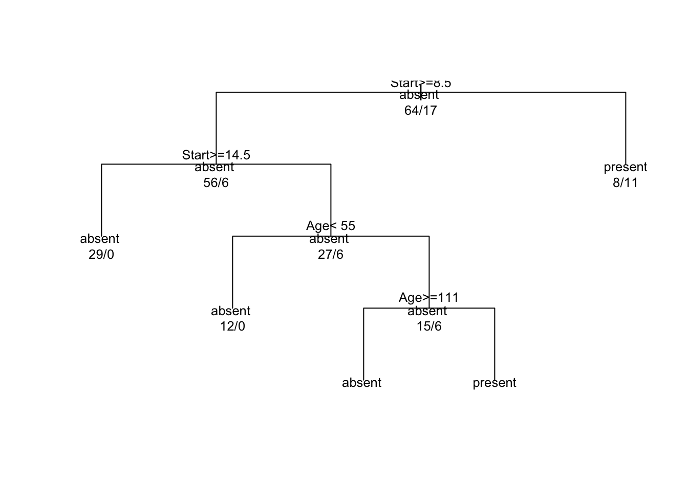
12.7 C4.5 Classifier
This classifier also follows recursive partitioning as in the previous case, but instead of minimizing the sum of squared errors between the sample data \(x\) and the true value \(p\) at each level, here the goal is to minimize entropy. This improves the information gain. Natural entropy (\(H\)) of the data \(x\) is defined as
\[ H = -\sum_x\; f(x) \cdot ln \;f(x) \]
where \(f(x)\) is the probability density of \(x\). This is intuitive because after the optimal split in recursing down the tree, the distribution of \(x\) becomes narrower, lowering entropy. This measure is also often known as ``differential entropy.’’
To see this let’s do a quick example. We compute entropy for two distributions of varying spread (standard deviation).
dx = 0.001
x = seq(-5,5,dx)
H2 = -sum(dnorm(x,sd=2)*log(dnorm(x,sd=2))*dx)
print(H2)
## [1] 2.042076H3 = -sum(dnorm(x,sd=3)*log(dnorm(x,sd=3))*dx)
print(H3)## [1] 2.111239Therefore, we see that entropy increases as the normal distribution becomes wider.
library(RWeka)
data(iris)
print(head(iris))
res = J48(Species~.,data=iris)
print(res)
summary(res)
12.8 Regression Trees
We move from classification trees (discrete outcomes) to regression trees (scored or continuous outcomes). Again, we use an example that already exists in R, i.e., the cars dataset in the cu.summary data frame. Let’s load it up.
data(cu.summary)
print(names(cu.summary))
## [1] "Price" "Country" "Reliability" "Mileage" "Type"print(head(cu.summary))## Price Country Reliability Mileage Type
## Acura Integra 4 11950 Japan Much better NA Small
## Dodge Colt 4 6851 Japan <NA> NA Small
## Dodge Omni 4 6995 USA Much worse NA Small
## Eagle Summit 4 8895 USA better 33 Small
## Ford Escort 4 7402 USA worse 33 Small
## Ford Festiva 4 6319 Korea better 37 Smallprint(tail(cu.summary))## Price Country Reliability Mileage Type
## Ford Aerostar V6 12267 USA average 18 Van
## Mazda MPV V6 14944 Japan Much better 19 Van
## Mitsubishi Wagon 4 14929 Japan <NA> 20 Van
## Nissan Axxess 4 13949 Japan <NA> 20 Van
## Nissan Van 4 14799 Japan <NA> 19 Van
## Volkswagen Vanagon 4 14080 Germany <NA> NA Vanprint(dim(cu.summary))## [1] 117 5print(unique(cu.summary$Type))## [1] Small Sporty Compact Medium Large Van
## Levels: Compact Large Medium Small Sporty Vanprint(unique(cu.summary$Country))## [1] Japan USA Korea Japan/USA Mexico Brazil Germany
## [8] France Sweden England
## 10 Levels: Brazil England France Germany Japan Japan/USA Korea ... USAWe will try and predict Mileage using the other variables. (Note: if we tried to predict Reliability, then we would be back in the realm of classification trees, here we are looking at regression trees.)
library(rpart)
fit <- rpart(Mileage~Price + Country + Reliability + Type, method="anova", data=cu.summary)
print(summary(fit))
## Call:
## rpart(formula = Mileage ~ Price + Country + Reliability + Type,
## data = cu.summary, method = "anova")
## n=60 (57 observations deleted due to missingness)
##
## CP nsplit rel error xerror xstd
## 1 0.62288527 0 1.0000000 1.0278364 0.17665513
## 2 0.13206061 1 0.3771147 0.5199982 0.10233496
## 3 0.02544094 2 0.2450541 0.4095695 0.08549195
## 4 0.01160389 3 0.2196132 0.4195450 0.09312124
## 5 0.01000000 4 0.2080093 0.4171213 0.08786038
##
## Variable importance
## Price Type Country
## 48 42 10
##
## Node number 1: 60 observations, complexity param=0.6228853
## mean=24.58333, MSE=22.57639
## left son=2 (48 obs) right son=3 (12 obs)
## Primary splits:
## Price < 9446.5 to the right, improve=0.6228853, (0 missing)
## Type splits as LLLRLL, improve=0.5044405, (0 missing)
## Reliability splits as LLLRR, improve=0.1263005, (11 missing)
## Country splits as --LRLRRRLL, improve=0.1243525, (0 missing)
## Surrogate splits:
## Type splits as LLLRLL, agree=0.950, adj=0.750, (0 split)
## Country splits as --LLLLRRLL, agree=0.833, adj=0.167, (0 split)
##
## Node number 2: 48 observations, complexity param=0.1320606
## mean=22.70833, MSE=8.498264
## left son=4 (23 obs) right son=5 (25 obs)
## Primary splits:
## Type splits as RLLRRL, improve=0.43853830, (0 missing)
## Price < 12154.5 to the right, improve=0.25748500, (0 missing)
## Country splits as --RRLRL-LL, improve=0.13345700, (0 missing)
## Reliability splits as LLLRR, improve=0.01637086, (10 missing)
## Surrogate splits:
## Price < 12215.5 to the right, agree=0.812, adj=0.609, (0 split)
## Country splits as --RRLRL-RL, agree=0.646, adj=0.261, (0 split)
##
## Node number 3: 12 observations
## mean=32.08333, MSE=8.576389
##
## Node number 4: 23 observations, complexity param=0.02544094
## mean=20.69565, MSE=2.907372
## left son=8 (10 obs) right son=9 (13 obs)
## Primary splits:
## Type splits as -LR--L, improve=0.515359600, (0 missing)
## Price < 14962 to the left, improve=0.131259400, (0 missing)
## Country splits as ----L-R--R, improve=0.007022107, (0 missing)
## Surrogate splits:
## Price < 13572 to the right, agree=0.609, adj=0.1, (0 split)
##
## Node number 5: 25 observations, complexity param=0.01160389
## mean=24.56, MSE=6.4864
## left son=10 (14 obs) right son=11 (11 obs)
## Primary splits:
## Price < 11484.5 to the right, improve=0.09693168, (0 missing)
## Reliability splits as LLRRR, improve=0.07767167, (4 missing)
## Type splits as L--RR-, improve=0.04209834, (0 missing)
## Country splits as --LRRR--LL, improve=0.02201687, (0 missing)
## Surrogate splits:
## Country splits as --LLLL--LR, agree=0.80, adj=0.545, (0 split)
## Type splits as L--RL-, agree=0.64, adj=0.182, (0 split)
##
## Node number 8: 10 observations
## mean=19.3, MSE=2.21
##
## Node number 9: 13 observations
## mean=21.76923, MSE=0.7928994
##
## Node number 10: 14 observations
## mean=23.85714, MSE=7.693878
##
## Node number 11: 11 observations
## mean=25.45455, MSE=3.520661
##
## n=60 (57 observations deleted due to missingness)
##
## node), split, n, deviance, yval
## * denotes terminal node
##
## 1) root 60 1354.58300 24.58333
## 2) Price>=9446.5 48 407.91670 22.70833
## 4) Type=Large,Medium,Van 23 66.86957 20.69565
## 8) Type=Large,Van 10 22.10000 19.30000 *
## 9) Type=Medium 13 10.30769 21.76923 *
## 5) Type=Compact,Small,Sporty 25 162.16000 24.56000
## 10) Price>=11484.5 14 107.71430 23.85714 *
## 11) Price< 11484.5 11 38.72727 25.45455 *
## 3) Price< 9446.5 12 102.91670 32.08333 *plot(fit, uniform=TRUE)
text(fit, use.n=TRUE, all=TRUE, cex=.8)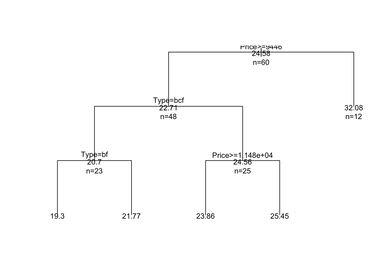
12.8.1 Example: Califonia Home Data
This example is taken from a data set posted by Cosmo Shalizi at CMU. We use a different package here, called tree, though this has been subsumed in most of its functionality by rpart used earlier. The analysis is as follows:
library(tree)
cahomes = read.table("DSTMAA_data/cahomedata.txt",header=TRUE)
print(dim(cahomes))
## [1] 20640 9head(cahomes)## MedianHouseValue MedianIncome MedianHouseAge TotalRooms TotalBedrooms
## 1 452600 8.3252 41 880 129
## 2 358500 8.3014 21 7099 1106
## 3 352100 7.2574 52 1467 190
## 4 341300 5.6431 52 1274 235
## 5 342200 3.8462 52 1627 280
## 6 269700 4.0368 52 919 213
## Population Households Latitude Longitude
## 1 322 126 37.88 -122.23
## 2 2401 1138 37.86 -122.22
## 3 496 177 37.85 -122.24
## 4 558 219 37.85 -122.25
## 5 565 259 37.85 -122.25
## 6 413 193 37.85 -122.25summary(cahomes)## MedianHouseValue MedianIncome MedianHouseAge TotalRooms
## Min. : 14999 Min. : 0.4999 Min. : 1.00 Min. : 2
## 1st Qu.:119600 1st Qu.: 2.5634 1st Qu.:18.00 1st Qu.: 1448
## Median :179700 Median : 3.5348 Median :29.00 Median : 2127
## Mean :206856 Mean : 3.8707 Mean :28.64 Mean : 2636
## 3rd Qu.:264725 3rd Qu.: 4.7432 3rd Qu.:37.00 3rd Qu.: 3148
## Max. :500001 Max. :15.0001 Max. :52.00 Max. :39320
## TotalBedrooms Population Households Latitude
## Min. : 1.0 Min. : 3 Min. : 1.0 Min. :32.54
## 1st Qu.: 295.0 1st Qu.: 787 1st Qu.: 280.0 1st Qu.:33.93
## Median : 435.0 Median : 1166 Median : 409.0 Median :34.26
## Mean : 537.9 Mean : 1425 Mean : 499.5 Mean :35.63
## 3rd Qu.: 647.0 3rd Qu.: 1725 3rd Qu.: 605.0 3rd Qu.:37.71
## Max. :6445.0 Max. :35682 Max. :6082.0 Max. :41.95
## Longitude
## Min. :-124.3
## 1st Qu.:-121.8
## Median :-118.5
## Mean :-119.6
## 3rd Qu.:-118.0
## Max. :-114.3mhv = as.matrix(as.numeric(cahomes$MedianHouseValue))
logmhv = log(mhv)
lat = as.matrix(as.numeric(cahomes$Latitude))
lon = as.matrix(as.numeric(cahomes$Longitude))
summary(lm(mhv~lat+lon))##
## Call:
## lm(formula = mhv ~ lat + lon)
##
## Residuals:
## Min 1Q Median 3Q Max
## -316022 -67502 -22903 46042 483381
##
## Coefficients:
## Estimate Std. Error t value Pr(>|t|)
## (Intercept) -5829397.0 82092.2 -71.01 <2e-16 ***
## lat -69551.0 859.6 -80.91 <2e-16 ***
## lon -71209.4 916.4 -77.70 <2e-16 ***
## ---
## Signif. codes: 0 '***' 0.001 '**' 0.01 '*' 0.05 '.' 0.1 ' ' 1
##
## Residual standard error: 100400 on 20637 degrees of freedom
## Multiple R-squared: 0.2424, Adjusted R-squared: 0.2423
## F-statistic: 3302 on 2 and 20637 DF, p-value: < 2.2e-16fit = tree(logmhv~lon+lat)
plot(fit)
text(fit,cex=0.8)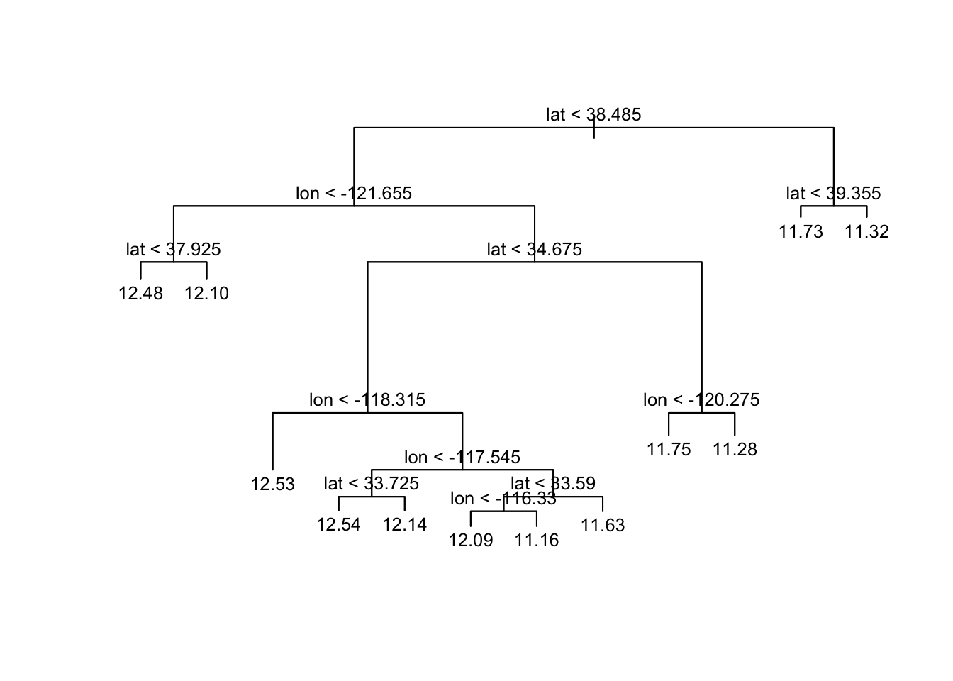
price.deciles = quantile(mhv,0:10/10)

cut.prices = cut(mhv,price.deciles,include.lowest=TRUE)
plot(lon, lat, col=grey(10:2/11)[cut.prices],pch=20,xlab="Longitude",ylab="Latitude")
partition.tree(fit,ordvars=c("lon","lat"),add=TRUE,cex=0.8)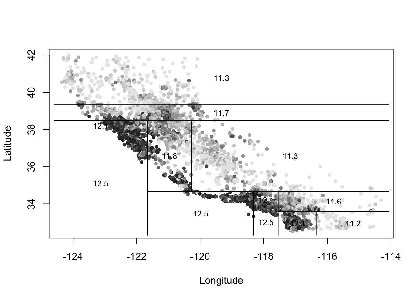
12.9 Random Forests
A random forest model is an extension of the CART class of models. In CART, at each decision node, all variables in the feature set are selected and the best one is determined for the bifurcation rule at that node. This approach tends to overfit the model to training data.
To ameliorate overfitting Breiman (2001) suggested generating classification and regression trees using a random subset of the feature set at each. One at a time, a random tree is grown. By building a large set of random trees (the default number in R is 500), we get a “random forest” of decision trees, and when the algorithm is run, each tree in the forest classifies the input. The output classification is determined by taking the modal classification across all trees.
The default number of variables from a feature set of \(p\) variables is defaulted to \(p/3\), rounded down, for a regression tree, and \(\sqrt{p}\) for a classification tree.
Reference: Breiman (2001)
For the NCAA data, take the top 32 teams and make their dependent variable 1, and that of the bottom 32 teams zero.
ncaa = read.table("DSTMAA_data/ncaa.txt",header=TRUE)

y1 = 1:32
y1 = y1*0+1
y2 = y1*0
y = c(y1,y2)
print(y)
## [1] 1 1 1 1 1 1 1 1 1 1 1 1 1 1 1 1 1 1 1 1 1 1 1 1 1 1 1 1 1 1 1 1 0 0 0
## [36] 0 0 0 0 0 0 0 0 0 0 0 0 0 0 0 0 0 0 0 0 0 0 0 0 0 0 0 0 0x = as.matrix(ncaa[4:14])library(randomForest)## randomForest 4.6-12## Type rfNews() to see new features/changes/bug fixes.yf = factor(y)
res = randomForest(x,yf)
print(res)##
## Call:
## randomForest(x = x, y = yf)
## Type of random forest: classification
## Number of trees: 500
## No. of variables tried at each split: 3
##
## OOB estimate of error rate: 28.12%
## Confusion matrix:
## 0 1 class.error
## 0 24 8 0.2500
## 1 10 22 0.3125print(importance(res))## MeanDecreaseGini
## PTS 4.625922
## REB 1.605147
## AST 1.999855
## TO 3.882536
## A.T 3.880554
## STL 2.026178
## BLK 1.951694
## PF 1.756469
## FG 4.159391
## FT 3.258861
## X3P 2.354894res = randomForest(x,yf,mtry=3)
print(res)##
## Call:
## randomForest(x = x, y = yf, mtry = 3)
## Type of random forest: classification
## Number of trees: 500
## No. of variables tried at each split: 3
##
## OOB estimate of error rate: 31.25%
## Confusion matrix:
## 0 1 class.error
## 0 23 9 0.28125
## 1 11 21 0.34375print(importance(res))## MeanDecreaseGini
## PTS 4.576616
## REB 1.379877
## AST 2.158874
## TO 3.847833
## A.T 3.674293
## STL 1.983024
## BLK 2.089959
## PF 1.621722
## FG 4.408469
## FT 3.562817
## X3P 2.19114312.10 Top Ten Algorithms in Data Science
The top voted algorithms in machine learning are: C4.5, k-means, SVM, Apriori, EM, PageRank, AdaBoost, kNN, Naive Bayes, CART. (This is just from one source, and differences of opinion will remain.)
12.11 Boosting
Boosting is an immensely popular machine learning technique. It is an iterative approach that takes weak learning algorithms and “boosts” them into strong learners. The method is intuitive. Start out with a classification algorithm such as logit for binary classification and run one pass to fit the model. Check which cases are correctly predicted in-sample, and which are incorrect. In the next classification pass (also known as a round), reweight the misclassified observations versus the correctly classified ones, by overweighting the former, and underweighting the latter. This forces the learner to “focus” more on the tougher cases, and adjust so that it gets these classified more accurately. Through multiple rounds, the results are boosted to higher levels of accuracy. Because there are many different weighting schemes, data scientists have evolved many different boosting algorithms. AdaBoost is one such popular algorithm, developed by Schapire and Singer (1999).
In recent times, these boosting algorithms have improved in their computer implementation, mostly through parallelization to speed them up when using huge data sets. Such versions are known as “extreme gradient” boosting algorithms. In R, the package xgboost contains an easy to use implementation. We illustrate with an example.
We use the sample data that comes with the xgboost package. Read in the data for the model.
library(xgboost)## Warning: package 'xgboost' was built under R version 3.3.2data("agaricus.train")
print(names(agaricus.train))## [1] "data" "label"print(dim(agaricus.train$data))## [1] 6513 126print(length(agaricus.train$label))## [1] 6513data("agaricus.test")
print(names(agaricus.test))## [1] "data" "label"print(dim(agaricus.test$data))## [1] 1611 126print(length(agaricus.test$label))## [1] 1611Fit the model. All that is needed is a single-line call to the xgboost function.
res = xgboost(data=agaricus.train$data, label=agaricus.train$label, objective = "binary:logistic", nrounds=5)## [1] train-error:0.000614
## [2] train-error:0.001228
## [3] train-error:0.000614
## [4] train-error:0.000614
## [5] train-error:0.000000print(names(res))## [1] "handle" "raw" "niter" "evaluation_log"
## [5] "call" "params" "callbacks"Undertake prediction using the predict function and then examine the confusion matrix for performance.
#In sample
yhat = predict(res,agaricus.train$data)
print(head(yhat,50))
## [1] 0.8973738 0.1030030 0.1030030 0.8973738 0.1018238 0.1030030 0.1030030
## [8] 0.8973738 0.1030030 0.1030030 0.1030030 0.1030030 0.1018238 0.1058771
## [15] 0.1018238 0.8973738 0.8973738 0.8973738 0.1030030 0.8973738 0.1030030
## [22] 0.1030030 0.8973738 0.1030030 0.1030030 0.8973738 0.1030030 0.1057071
## [29] 0.1030030 0.1144627 0.1058771 0.1139800 0.1030030 0.1057071 0.1058771
## [36] 0.1030030 0.1030030 0.1030030 0.1030030 0.1057071 0.1057071 0.1030030
## [43] 0.1030030 0.8973738 0.1030030 0.1030030 0.1057071 0.1058771 0.1030030
## [50] 0.1030030cm = table(agaricus.train$label,as.integer(round(yhat)))
print(cm)##
## 0 1
## 0 3373 0
## 1 0 3140print(chisq.test(cm))##
## Pearson's Chi-squared test with Yates' continuity correction
##
## data: cm
## X-squared = 6509, df = 1, p-value < 2.2e-16#Out of sample
yhat = predict(res,agaricus.test$data)
print(head(yhat,50))## [1] 0.1030030 0.8973738 0.1030030 0.1030030 0.1058771 0.1139800 0.8973738
## [8] 0.1030030 0.8973738 0.1057071 0.8973738 0.1030030 0.1018238 0.1030030
## [15] 0.1018238 0.1057071 0.1030030 0.8973738 0.1058771 0.1030030 0.1030030
## [22] 0.1057071 0.1030030 0.1030030 0.1057071 0.8973738 0.1139800 0.1030030
## [29] 0.1030030 0.1018238 0.1030030 0.1030030 0.1057071 0.1058771 0.1030030
## [36] 0.1030030 0.1139800 0.8973738 0.1030030 0.1030030 0.1058771 0.1030030
## [43] 0.1030030 0.1030030 0.1030030 0.1144627 0.1057071 0.1144627 0.1058771
## [50] 0.1030030cm = table(agaricus.test$label,as.integer(round(yhat)))
print(cm)##
## 0 1
## 0 835 0
## 1 0 776print(chisq.test(cm))##
## Pearson's Chi-squared test with Yates' continuity correction
##
## data: cm
## X-squared = 1607, df = 1, p-value < 2.2e-16There are many types of algorithms that may be used with boosting, see the documentation of the function in R. But here are some of the options.
- reg:linear, linear regression (Default).
- reg:logistic, logistic regression.
- binary:logistic, logistic regression for binary classification. Output probability.
- binary:logitraw, logistic regression for binary classification, output score before logistic transformation.
- multi:softmax, set xgboost to do multiclass classification using the softmax objective. Class is represented by a number and should be from 0 to num_class - 1.
- multi:softprob, same as softmax, but prediction outputs a vector of ndata * nclass elements, which can be further reshaped to ndata, nclass matrix. The result contains predicted probabilities of each data point belonging to each class.
- rank:pairwise set xgboost to do ranking task by minimizing the pairwise loss.
Let’s repeat the exercise using the NCAA data.
ncaa = read.table("DSTMAA_data/ncaa.txt",header=TRUE)
y = as.matrix(c(rep(1,32),rep(0,32)))
x = as.matrix(ncaa[4:14])
res = xgboost(data=x,label=y,objective = "binary:logistic", nrounds=10)
## [1] train-error:0.109375
## [2] train-error:0.062500
## [3] train-error:0.031250
## [4] train-error:0.046875
## [5] train-error:0.046875
## [6] train-error:0.031250
## [7] train-error:0.015625
## [8] train-error:0.015625
## [9] train-error:0.015625
## [10] train-error:0.000000yhat = predict(res,x)
print(yhat)## [1] 0.93651539 0.91299230 0.94973743 0.92731959 0.88483542 0.78989410
## [7] 0.87560666 0.90532523 0.86085796 0.83430755 0.91133112 0.77964365
## [13] 0.65978771 0.91299230 0.93371087 0.91403663 0.78532064 0.80347157
## [19] 0.60545647 0.79564470 0.84763408 0.86694145 0.79334742 0.91165835
## [25] 0.80980736 0.76779360 0.90779346 0.88314682 0.85020524 0.77409834
## [31] 0.85503411 0.92695338 0.49809304 0.15059802 0.13718443 0.30433667
## [37] 0.35902274 0.08057866 0.16935477 0.06189578 0.08516480 0.12777112
## [43] 0.06224639 0.18913418 0.07675765 0.33156753 0.06586388 0.13792981
## [49] 0.22327985 0.08479820 0.16396984 0.10236575 0.16346745 0.27498406
## [55] 0.10642117 0.07299758 0.15809764 0.15259050 0.07768227 0.15006000
## [61] 0.08349544 0.06932075 0.10376420 0.11887703cm = table(y,as.integer(round(yhat)))
print(cm)##
## y 0 1
## 0 32 0
## 1 0 32print(chisq.test(cm))##
## Pearson's Chi-squared test with Yates' continuity correction
##
## data: cm
## X-squared = 60.062, df = 1, p-value = 9.189e-15References
Breiman, Leo. 2001. “Random Forests.” Mach. Learn. 45 (1). Hingham, MA, USA: Kluwer Academic Publishers: 5–32. doi:10.1023/A:1010933404324.
Schapire, Robert E., and Yoram Singer. 1999. “Improved Boosting Algorithms Using Confidence-Rated Predictions.” In Machine Learning, 80–91.