Chapter 1 The Art of Data Science
“All models are wrong, but some are useful.” — George E. P. Box and N.R. Draper in “Empirical Model Building and Response Surfaces,” John Wiley & Sons, New York, 1987.
So you want to be a “data scientist”? There is no widely accepted definition of who a data scientist is.1 Several books now attempt to define what data science is and who a data scientist may be, see Patil (2012), Patil (2011), and Loukides (2012). This book’s viewpoint is that a data scientist is someone who asks unique, interesting questions of data based on formal or informal theory, to generate rigorous and useful insights.2 It is likely to be an individual with multi-disciplinary training in computer science, business, economics, statistics, and armed with the necessary quantity of domain knowledge relevant to the question at hand. The potential of the field is enormous for just a few well-trained data scientists armed with big data have the potential to transform organizations and societies. In the narrower domain of business life, the role of the data scientist is to generate applicable business intelligence.
Among all the new buzzwords in business – and there are many – “Big Data” is one of the most often heard. The burgeoning social web, and the growing role of the internet as the primary information channel of business, has generated more data than we might imagine. Users upload an hour of video data to YouTube every second.3 87% of the U.S. population has heard of Twitter, and 7% use it.4 Forty-nine percent of Twitter users follow some brand or the other, hence the reach is enormous, and, as of 2014, there are more then 500 million tweets a day. But data is not information, and until we add analytics, it is just noise. And more, bigger, data may mean more noise and does not mean better data.
In many cases, less is more, and we need models as well. That is what this book is about, it’s about theories and models, with or without data, big or small. It’s about analytics and applications, and a scientific approach to using data based on well-founded theory and sound business judgment. This book is about the science and art of data analytics.
Data science is transforming business. Companies are using medical data and claims data to offer incentivized health programs to employees. Caesar’s Entertainment Corp. analyzed data for 65,000 employees and found substantial cost savings. Zynga Inc, famous for its game Farmville, accumulates 25 terabytes of data every day and analyzes it to make choices about new game features. UPS installed sensors to collect data on speed and location of its vans, which combined with GPS information, reduced fuel usage in 2011 by 8.4 million gallons, and shaved 85 million miles off its routes.5 McKinsey argues that a successful data analytics plan contains three elements: interlinked data inputs, analytics models, and decision-support tools.6 In a seminal paper, Halevy, Norvig, and Pereira (2009) argue that even simple theories and models, with big data, have the potential to do better than complex models with less data.
In a recent talk7 well-regarded data scientist Hilary Mason emphasized that the creation of “data products” requires three components: data (of course) plus technical expertise (machine-learning) plus people and process (talent). Google Maps is a great example of a data product that epitomizes all these three qualities. She mentioned three skills that good data scientists need to cultivate: (a) in math and stats, (b) coding, (c) communication. I would add that preceding all these is the ability to ask relevant questions, the answers to which unlock value for companies, consumers, and society. Everything in data analytics begins with a clear problem statement, and needs to be judged with clear metrics.
Being a data scientist is inherently interdisciplinary. Good questions come from many disciplines, and the best answers are likely to come from people who are interested in multiple fields, or at least from teams that co-mingle varied skill sets. Josh Wills of Cloudera stated it well - “A data scientist is a person who is better at statistics than any software engineer and better at software engineering than any statistician.” In contrast, complementing data scientists are business analytics people, who are more familiar with business models and paradigms and can ask good questions of the data.
1.1 Volume, Velocity, Variety
There are several “V”s of big data: three of these are volume, velocity, variety.8 Big data exceeds the storage capacity of conventional databases. This is it’s volume aspect. The scale of data generation is mind-boggling. Google’s Eric Schmidt pointed out that until 2003, all of human kind had generated just 5 exabytes of data (an exabyte is \(1000^6\) bytes or a billion-billion bytes). Today we generate 5 exabytes of data every two days. The main reason for this is the explosion of “interaction” data, a new phenomenon in contrast to mere “transaction” data. Interaction data comes from recording activities in our day-to-day ever more digital lives, such as browser activity, geo-location data, RFID data, sensors, personal digital recorders such as the fitbit and phones, satellites, etc. We now live in the “internet of things” (or iOT), and it’s producing a wild quantity of data, all of which we seem to have an endless need to analyze. In some quarters it is better to speak of 4 Vs of big data, as shown in Figure 1.1.
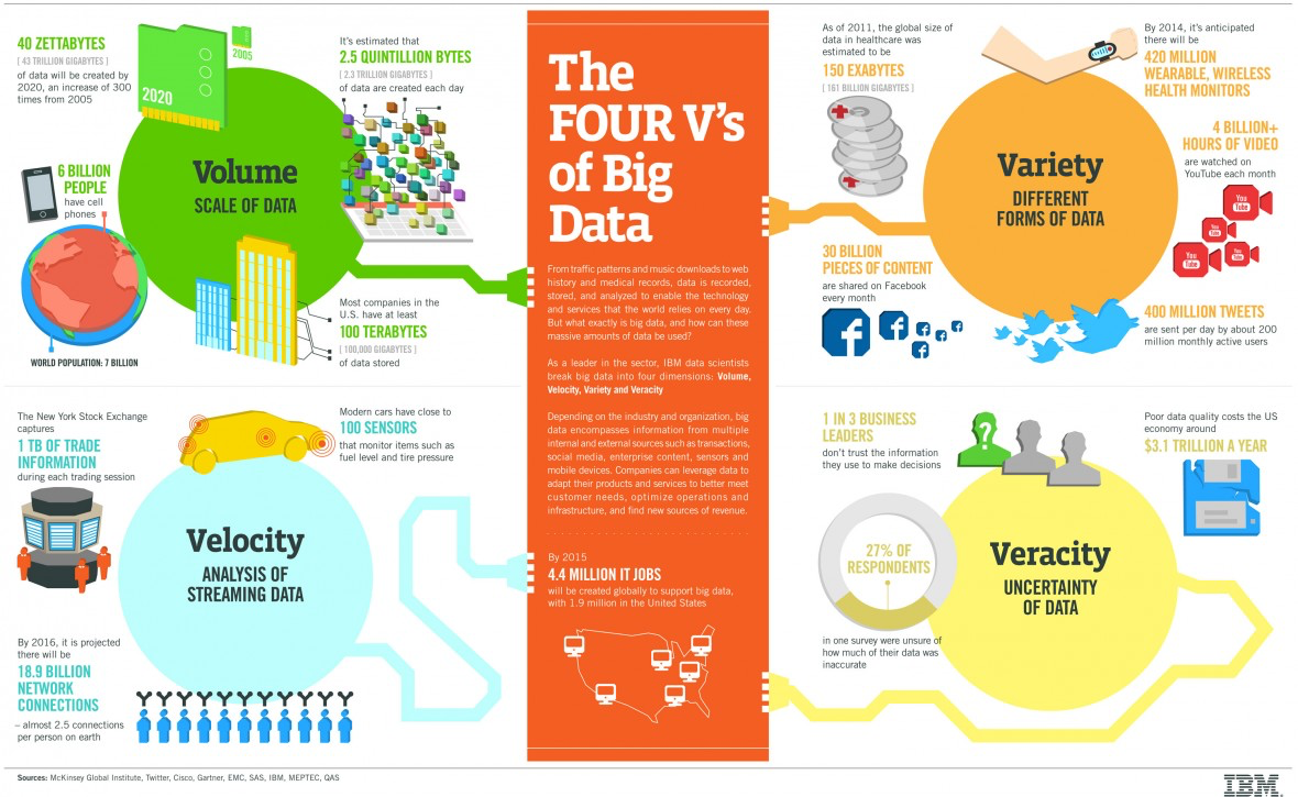
Figure 1.1: The Four Vs of Big Data
A good data scientist will be adept at managing volume not just technically in a database sense, but by building algorithms to make intelligent use of the size of the data as efficiently as possible. Things change when you have gargantuan data because almost all correlations become significant, and one might be tempted to draw spurious conclusions about causality. For many modern business applications today extraction of correlation is sufficient, but good data science involves techniques that extract causality from these correlations as well.
In many cases, detecting correlations is useful as is. For example, consider the classic case of Google Flu Trends, see Figure 1.2. The figure shows the high correlation between flu incidence and searches about “flu” on Google, see Ginsberg et al. (2009); Culotta (2010). Obviously searches on the key word “flu” do not result in the flu itself! Of course, the incidence of searches on this key word is influenced by flu outbreaks. The interesting point here is that even though searches about flu do not cause flu, they correlate with it, and may at times even be predictive of it, simply because searches lead the actual reported levels of flu, as those may occur concurrently but take time to be reported. And whereas searches may be predictive, the cause of searches is the flu itself, one variable feeding on the other, in a repeat cycle.9 Hence, prediction is a major outcome of correlation, and has led to the recent buzz around the subfield of “predictive analytics.” There are entire conventions devoted to this facet of correlation, such as the wildly popular PAW (Predictive Analytics World).10 Pattern recognition is in, passe causality is out.
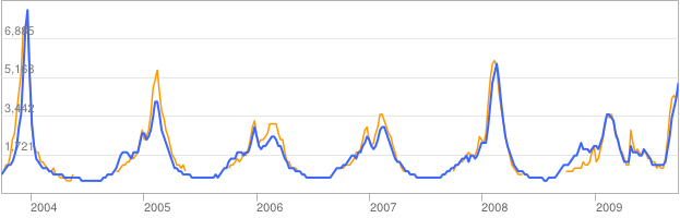
Figure 1.2: Google Flu Trends. The figure shows the high correlation between flu incidence and searches about “flu” on Google. The orange line is actual US flu activity, and the blue line is the Google Flu Trends estimate.
Data velocity is accelerating. Streams of tweets, Facebook entries, financial information, etc., are being generated by more users at an ever increasing pace. Whereas velocity increases data volume, often exponentially, it might shorten the window of data retention or application. For example, high-frequency trading relies on micro-second information and streams of data, but the relevance of the data rapidly decays.
Finally, data variety is much greater than ever before. Models that relied on just a handful of variables can now avail of hundreds of variables, as computing power has increased. The scale of change in volume, velocity, and variety of the data that is now available calls for new econometrics, and a range of tools for even single questions. This book aims to introduce the reader to a variety of modeling concepts and econometric techniques that are essential for a well-rounded data scientist.
Data science is more than the mere analysis of large data sets. It is also about the creation of data. The field of “text-mining” expands available data enormously, since there is so much more text being generated than numbers. The creation of data from varied sources, and its quantification into information is known as “datafication.”
1.2 Machine Learning
Data science is also more than “machine learning,” which is about how systems learn from data. Systems may be trained on data to make decisions, and training is a continuous process, where the system updates its learning and (hopefully) improves its decision-making ability with more data. A spam filter is a good example of machine learning. As we feed it more data it keeps changing its decision rules, using a Bayesian filter, thereby remaining ahead of the spammers. It is this ability to adaptively learn that prevents spammers from gaming the filter, as highlighted in Paul Graham’s interesting essay titled “A Plan for Spam.”11 Credit card approvals are also based on neural-nets, another popular machine learning technique. However, machine-learning techniques favor data over judgment, and good data science requires a healthy mix of both. Judgment is needed to accurately contextualize the setting for analysis and to construct effective models. A case in point is Vinny Bruzzese, known as the “mad scientist of Hollywood” who uses machine learning to predict movie revenues.12 He asserts that mere machine learning would be insufficient to generate accurate predictions. He complements machine learning with judgment generated from interviews with screenwriters, surveys, etc., “to hear and understand the creative vision, so our analysis can be contextualized.”
Machine intelligence is re-emerging as the new incarnation of AI (a field that many feel has not lived up to its promise). Machine learning promises and has delivered on many questions of interest, and is also proving to be quite a game-changer, as we will see later on in this chapter, and also as discussed in many preceding examples. What makes it so appealing? Hilary Mason suggests four characteristics of machine intelligence that make it interesting: (i) It is usually based on a theoretical breakthrough and is therefore well grounded in science. (ii) It changes the existing economic paradigm. (iii) The result is commoditization (e.g. Hadoop), and (iv) it makes available new data that leads to further data science.
Machine Learning (a.k.a. “ML”) has diverged and is now defined separate from traditional statistics. ML is more about learning and matching inputs with outputs, whereas statistics has always been interested more in analyzing data under a given problem statement or hypothesis. ML tends to be more heuristic, whereas econometrics and statistical analyses tend to be theory-driven, with tight assumptions. ML tends to focus more on prediction, econometrics on causality, which is a stronger outcome than prediction (or correlation). ML techniques work well with big data, whereas econometrics techniques tend toward too much significance with too much data. Hence, the latter is better served with dimension reduction, though ML may not in fact be implementable with small data. Under ML techniques, even when they work very well, it is hard to explain why, and also which variables in the feature set seem to work best. Under traditional econometrics and statistics, tracing the effects in the model is clear and feasible, making understanding of the model better. Deciding which approach fits a given problem best is a matter of taste, but experience often helps in deciding which one of the two methods applies better.
Let’s examine a definition of Machine Learning. Tom Mitchell, one of the founders of the field, stated a formal definition thus:
“A computer program is said to learn from experience \(E\) with respect to some class of tasks \(T\) and performance measure \(P\) if its performance at tasks in \(T\), as measured by \(P\), improves with experience \(E\).” – Mitchell (1997)
Domingos (2012) offers an excellent introductionmachine learning. He defines learning as the sum of Representation, Evaluation, and Optimization. Machine learning representation requires specifying the problem in a formal language that a computer can handle. These representations will differ for different machine learning techniques. For example, in a classification problem, there may be a choice of many classifiers, each of which will be formally represented. Next, a scoring function or a loss function is specified in order to complete the evaluation step. Finally, best evaluation is attained through optimization.
Once these steps have been undertaken and the best ML algorithm is chosen on the training data, we may validate the model on out-of-sample data, or the test data set. One may randomly choose a fraction of the data sample to hold out for validation. Repeating this process by holding out different parts of the data for testing, and training on the remainder, is a process known as cross-validation and is strongly recommended.
If it turns out that repeated cross-validation results in poor results, even though in-sample testing does very well, then it is possible evidence of over-fitting. Over-fitting usually occurs when the model is over-parameterized in-sample, so that it fits very well, but then it becomes less useful on new data. This is akin to driving by looking in the rear-view mirror, which does not work well when the road does not remain straight going forward. Therefore, many times, simpler and less parameterized models tend to work better in forecasting and prediction settings. If the model performs pretty much the same in-sample and out-of-sample, it is very unlikely to be overfit. The argument that simpler models overfit less is often made with Occam’s Razor in mind, but is not always an accurate underpinning, so simpler may not always be better.13
1.3 Supervised and Unsupervised Learning
Systems may learn in two broad ways, through “supervised” and “unsupervised” learning. In supervised learning, a system produces decisions (outputs) based on input data. Both spam filters and automated credit card approval systems are examples of this type of learning. So is linear discriminant analysis (LDA). The system is given a historical data sample of inputs and known outputs, and it “learns” the relationship between the two using machine learning techniques, of which there are several. Judgment is needed to decide which technique is most appropriate for the task at hand.
Unsupervised learning is a process of reorganizing and enhancing the inputs in order to place structure on unlabeled data. A good example is cluster analysis, which takes a collection of entities, each with a number of attributes, and partitions the entity space into sets or groups based on closeness of the attributes of all entities. What this does is reorganizes the data, but it also enhances the data through a process of labeling the data with additional tags (in this case a cluster number/name). Factor analysis is also an unsupervised learning technique. The origin of this terminology is unclear, but it presumably arises from the fact that there is no clear objective function that is maximized or minimized in unsupervised learning, so that no “supervision” to reach an optimal is called for. However, this is not necessarily true in general, and we will see examples of unsupervised learning (such as community detection in the social web) where the outcome depends on measurable objective criteria.
Supervised learning might include broad topics such as regression, classification, forecasting, and importance attribution. All these analyses are supported by the fact that the feature set (\(X\) variables) are accompanied by tags (\(Y\) variables). Unsupervised learning includes analyses such as clustering, and association models, e.g., recommendation engines, market baskets, etc.
1.4 Feature Selection
When faced with a machine learning problem, having the right data is paramount. Sometimes, especially in this age of Big Data, we may have too much data; abundance comes with a curse. Too much data also might mean featureless data, which is not useful to the data scientist. Hence, we might want to extract those data variables that are useful, through a process called “feature selection”. Dimension reduction is also a useful by product of feature selection, and pruning data might also mean that ML algorithms will run faster, and converge better.
Wikipedia defines feature selection as – “In machine learning and statistics, feature selection, also known as variable selection, attribute selection or variable subset selection, is the process of selecting a subset of relevant features (variables, predictors) for use in model construction.”14
Feature selection subsets the variable space. If there are \(p\) columns of data, then we choose \(q \ll p\) variates. Feature extraction on the other hand refers to transformation of the original variables to create new variables, i.e., functionals of \(p\), such as \(g(p)\). We will encounter these topics later on, as we work through various ML techniques.
1.5 Ensemble Learning
Ensemble models are simply combinations of many ML models. There are of course, many ways in which models may be combined to generate better ML models. It is astonishing how powerful this “model democracy” turns out to be where various models vote, for example, on a classification problem. In S. R. Das and Chen (2007), five different classifiers vote on classifying stock bulletin board messages into three categories of signals: Buy, Hold, Sell. In this early work, ensemble methods were able to improve the signal-to-noise ratio in classification.
Different classification models are not always necessary. One may instead calibrate the same model to different subsamples of the training data, delivering multiple similar, but different models. Each of these models is then used to classify out-of-sample, and the decision is made by voting across models. This method is known as bagging. One of the most popular examples of bagging algorithms is the random forest model, which we will encounter later when we examine classifiers in more detail.
In another technique, boosting, the loss function that is being optimized does not weight all examples in the training data set equally. After one pass of calibration, training examples are reweighted such that the cases where the ML algorithm made errors (as in a classification problem) are given higher weight in the loss function. By penalizing these observations, the algorithm learns to prevent those mistakes as they are more costly.
Another approach to ensemble learning is called stacking where models are chained to each other, so that the output of low-level models becomes the input of another higher-level model. Here models are vertically integrated in contrast to bagging, where models are horizontally integrated.
1.6 Predictions and Forecasts
Data science is about making predictions and forecasts. There is a difference between the two. The statistician-economist Paul Saffo has suggested that predictions aim to identify one outcome, whereas forecasts encompass a range of outcomes. To say that “it will rain tomorrow” is to make a prediction, but to say that “the chance of rain is 40%” (implying that the chance of no rain is 60%) is to make a forecast, as it lays out the range of possible outcomes with probabilities. We make weather forecasts, not predictions. Predictions are statements of great certainty, whereas forecasts exemplify the range of uncertainty. In the context of these definitions, the term predictive analytics is a misnomer for it’s goal is to make forecasts, not mere predictions.
1.7 Innovation and Experimentation
Data science is about new ideas and approaches. It merges new concepts with fresh algorithms. Take for example the A/B test, which is nothing but the online implementation of a real-time focus group. Different subsets of users are exposed to A and B stimuli respectively, and responses are measured and analyzed. It is widely used for web site design. This approach has been in place for more than a decade, and in 2011 Google ran more than 7,000 A/B tests. Facebook, Amazon, Netflix, and several others firms use A/B testing widely.15 The social web has become a teeming ecosystem for running social science experiments. The potential to learn about human behavior using innovative methods is much greater now than ever before.
1.8 The Dark Side
1.8.1 Big Errors
The good data scientist will take care to not over-reach in drawing conclusions from big data. Because there are so many variables available, and plentiful observations, correlations are often statistically significant, but devoid of basis. In the immortal words of the bard, empirical results from big data may be - “A tale told by an idiot, full of sound and fury, signifying nothing.”16 One must be careful not to read too much in the data. More data does not guarantee less noise, and signal extraction may be no easier than with less data.
Adding more columns (variables in the cross section) to the data set, but not more rows (time dimension) is also fraught with danger. As the number of variables increases, more characteristics are likely to be related statistically. Over fitting models in-sample is much more likely with big data, leading to poor performance out-of-sample.
Researchers have also to be careful to explore the data fully, and not terminate their research the moment a viable result, especially one that the researcher is looking for, is attained. With big data, the chances of stopping at a suboptimal, or worse, intuitively appealing albeit wrong result become very high. It is like asking a question to a class of students. In a very large college class, the chance that someone will provide a plausible yet off-base answer quickly is very high, which often short circuits the opportunity for others in class to think more deeply about the question and provide a much better answer.
Nassim Taleb17 describes these issues elegantly - “I am not saying there is no information in big data. There is plenty of information. The problem – the central issue – is that the needle comes in an increasingly larger haystack.” The fact is, one is not always looking for needles or Taleb’s black swans, and there are plenty of normal phenomena about which robust forecasts are made possible by the presence of big data.
1.8.2 Privacy
The emergence of big data coincides with a gigantic erosion of privacy. Human kind has always been torn between the need for social interaction, and the urge for solitude and privacy. One trades off against the other. Technology has simply sharpened the divide and made the slope of this trade off steeper. It has provided tools of social interaction that steal privacy much faster than in the days before the social web.
Rumors and gossip are now old world. They required bilateral transmission. The social web provides multilateral revelation, where privacy no longer capitulates a battle at a time, but the entire war is lost at one go. And data science is the tool that enables firms, governments, individuals, benefactors and predators, et al, en masse, to feed on privacy’s carcass. The cartoon in Figure 1.3 parodies the kind of information specialization that comes with the loss of privacy!
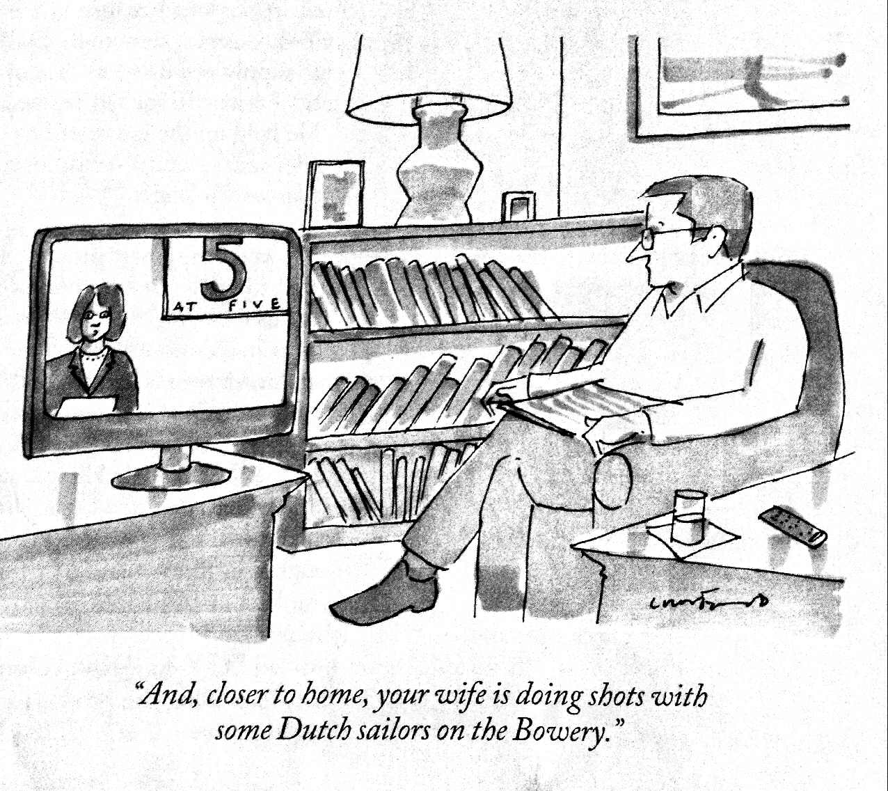
Figure 1.3: Profiling can convert mass media into personal media.
The loss of privacy is manifested in the practice of human profiling through data science. Our web presence increases entropically as we move more of our life’s interactions to the web, be they financial, emotional, organizational, or merely social. And as we live more and more of our lives in this new social melieu, data mining and analytics enables companies to construct very accurate profiles of who we are, often better than what we might do ourselves. We are moving from “know thyself” to knowing everything about almost everyone.
If you have a Facebook or Twitter presence, rest assured you have been profiled. For instance, let’s say you tweeted that you were taking your dog for a walk. Profiling software now increments your profile with an additional tag - pet owner. An hour later you tweet that you are returning home to cook dinner for your kids. You profile is now further tagged as a parent. As you might imagine, even a small Twitter presence ends up being dramatically revealing about who you are. Information that you provide on Facebook and Twitter, your credit card spending pattern, and your blog, allows the creation of a profile that is accurate and comprehensive, and probably more objective than the subjective and biased opinion that you have of yourself. A machine knows thyself better. And you are the product! (See Figure 1.4.)
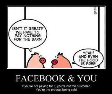
Figure 1.4: If its free, you may be the product.
Humankind leaves an incredible trail of “digital exhaust” comprising phone calls, emails, tweets, GPS information, etc., that companies use for profiling. It is said that 1/3 of people have a digital identity before being born, initiated with the first sonogram from a routine hospital visit by an expectant mother. The half life of non-digital identity, or the average age of digital birth is six months, and within two years 92% of the US population has a digital identity.18 Those of us who claim to be safe from revealing their privacy by avoiding all forms of social media are simply profiled as agents with a “low digital presence.” It might be interesting to ask such people whether they would like to reside in a profile bucket that is more likely to attract government interest than a profile bucket with more average digital presence. In this age of profiling, the best way to remain inconspicuous is not to hide, but to remain as average as possible, so as to be mostly lost within a large herd.
Privacy is intricately and intrinsically connected to security and efficiency. The increase in transacting on the web, and the confluence of profiling, has led to massive identity theft. Just as in the old days, when a thief picked your lock and entered your home, most of your possessions were at risk. It is the same with electronic break ins, except that there are many more doors to break in from and so many more windows through which an intruder can unearth revealing information. And unlike a thief who breaks into your home, a hacker can reside in your electronic abode for quite some time without being detected, an invisible parasite slowly doing damage. While you are blind, you are being robbed blind. And unlike stealing your worldly possessions, stealing your very persona and identity is the cruelest cut of them all.
An increase in efficiency in the web ecosystem comes too at some retrenchment of privacy. Who does not shop on the internet? Each transaction resides in a separate web account. These add up at an astonishing pace. I have no idea of the exact number of web accounts in my name, but I am pretty sure it is over a hundred, many of them used maybe just once. I have unconsciously, yet quite willingly, marked my territory all over the e-commerce landscape. I rationalize away this loss of privacy in the name of efficiency, which undoubtedly exists. Every now and then I am reminded of this loss of privacy as my plane touches down in New York city, and like clockwork, within an hour or two, I receive a discount coupon in my email from Barnes & Noble bookstores. You see, whenever I am in Manhattan, I frequent the B&N store on the upper west side, and my credit card company and/or Google knows this, as well as my air travel schedule, since I buy both tickets and books on the same card and in the same browser. So when I want to buy books at a store discount, I fly to New York. That’s how rational I am, or how rational my profile says I am! Humor aside, such profiling seems scary, though the thought quickly passes. I like the dopamine rush I get from my discount coupon and I love buying books.19
Profiling implies a partitioning of the social space into targeted groups, so that focused attention may be paid to specific groups, or various groups may be treated differently through price discrimination. If my profile shows me to be an affluent person who likes fine wine (both facts untrue in my case, but hope springs eternal), then internet sales pitches (via Groupon, Living Social, etc.) will be priced higher to me by an online retailer than to someone whose profile indicates a low spend. Profiling enables retailers to maximize revenues by eating away the consumer’s surplus by better setting of prices to each buyer’s individual willingness to pay. This is depicted in Figure 1.5.
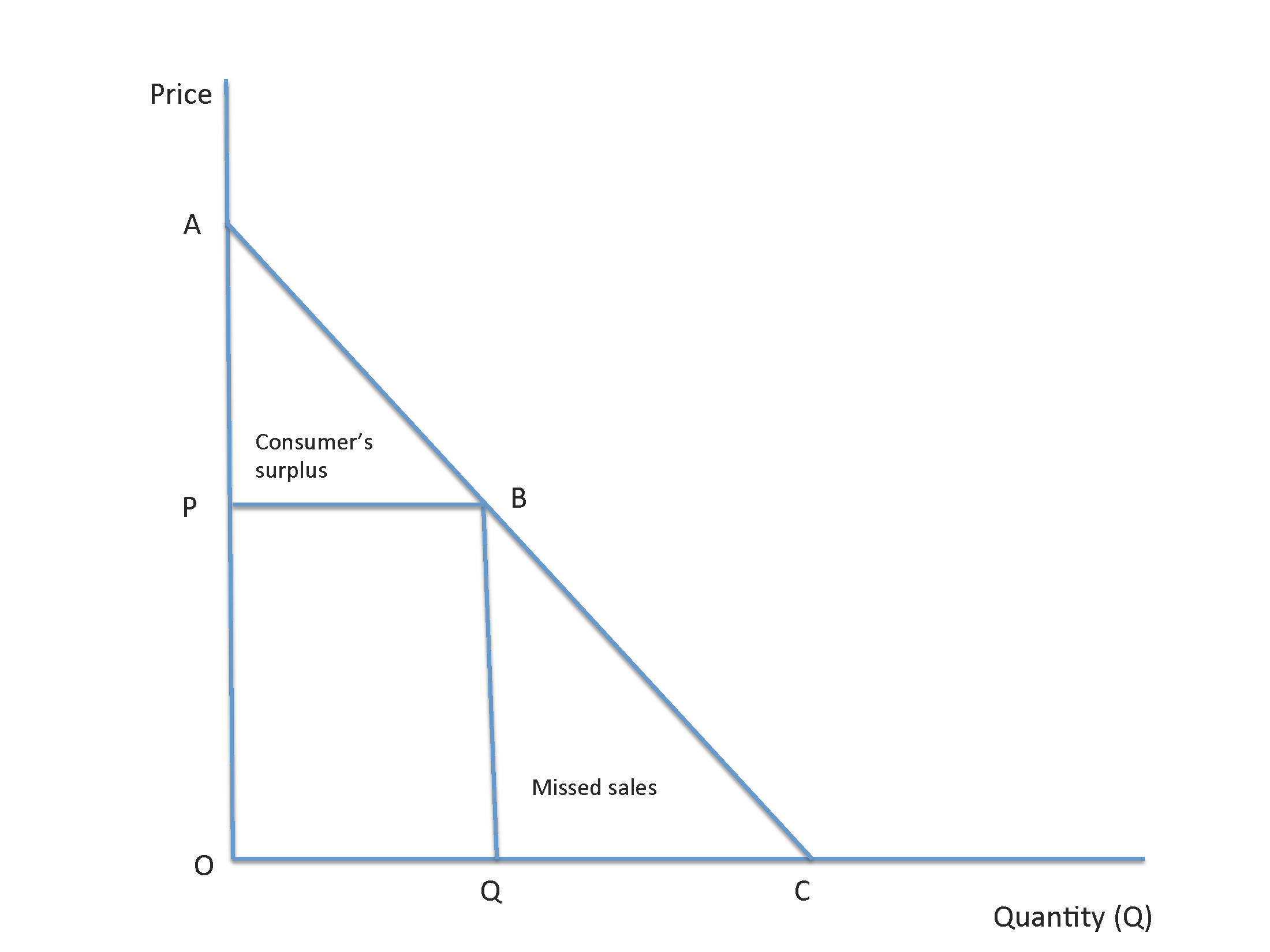
Figure 1.5: Extracting consumers surplus through profiling.
In Figure 1.5 the demand curve is represented by the line segment \(ABC\) representing price-quantity combinations (more is demanded at lower prices). In a competitive market without price segmentation, let’s assume that the equilibrium price is \(P\) and equilibrium quantity is \(Q\) as shown by the point \(B\) on the demand curve. (The upward sloping supply curve is not shown but it must intersect the demand curve at point \(B\), of course.) Total revenue to the seller is the area \(OPBQ\), i.e., \(P \times Q\).
Now assume that the seller is able to profile buyers so that price discrimination is possible. Based on buyers’ profiles, the seller will offer each buyer the price he is willing to pay on the demand curve, thereby picking off each price in the segment \(AB\). This enables the seller to capture the additional region \(ABP\), which is the area of consumer’s surplus, i.e., the difference between the price that buyers pay versus the price they were actually willing to pay. The seller may also choose to offer some consumers lower prices in the region \(BC\) of the demand curve so as to bring in additional buyers whose threshold price lies below the competitive market price \(P\). Thus, profiling helps sellers capture consumer’s surplus and eat into the region of missed sales. Targeting brings benefits to sellers and they actively pursue it. The benefits outweigh the costs of profiling, and the practice is widespread as a result. Profiling also makes price segmentation fine-tuned, and rather than break buyers into a few segments, usually two, each profile becomes a separate segment, and the granularity of price segmentation is modulated by the number of profiling groups the seller chooses to model.
Of course, there is an insidious aspect to profiling, which has existed for quite some time, such as targeting conducted by tax authorities. I don’t believe we will take kindly to insurance companies profiling us any more than they already do. Profiling is also undertaken to snare terrorists. However, there is a danger in excessive profiling. A very specific profile for a terrorist makes it easier for their ilk to game detection as follows. Send several possible suicide bombers through airport security and see who is repeatedly pulled aside for screening and who is not. Repeating this exercise enables a terrorist cell to learn which candidates do not fall into the profile. They may then use them for the execution of a terror act, as they are unlikely to be picked up for special screening. The antidote? Randomization of people picked for special screening in searches at airports, which makes it hard for a terrorist to always assume no likelihood of detection through screening.20
Automated invasions of privacy naturally lead to a human response, not always rational or predictable. This is articulated in Campbell’s Law: “The more any quantitative social indicator (or even some qualitative indicator) is used for social decision-making, the more subject it will be to corruption pressures and the more apt it will be to distort and corrupt the social processes it is intended to monitor.”21 We are in for an interesting period of interaction between man and machine, where the battle for privacy will take center stage.
1.9 Theories, Models, Intuition, Causality, Prediction, Correlation
My view of data science is one where theories are implemented using data, some of it big data. This is embodied in an inference stack comprising (in sequence): theories, models, intuition, causality, prediction, and correlation. The first three constructs in this chain are from Emanuel Derman’s wonderful book on the pitfalls of models.^[“Models. Behaving. Badly.” Emanuel Derman, Free Press, New York, 2011.}
Theories are statements of how the world should be or is, and are derived from axioms that are assumptions about the world, or precedent theories. Models are implementations of theory, and in data science are often algorithms based on theories that are run on data. The results of running a model lead to intuition, i.e., a deeper understanding of the world based on theory, model, and data. Whereas there are schools of thought that suggest data is all we need, and theory is obsolete, this author disagrees. Still the unreasonable proven effectiveness of big data cannot be denied. Chris Anderson argues in his Wired magazine article thus:“22
Sensors everywhere. Infinite storage. Clouds of processors. Our ability to capture, warehouse, and understand massive amounts of data is changing science, medicine, business, and technology. As our collection of facts and figures grows, so will the opportunity to find answers to fundamental questions. Because in the era of big data, more isn’t just more. More is different.
In contrast, the academic Thomas Davenport writes in his foreword to Siegel (2013) that models are key, and should not be increasingly eschewed with increasing data:
But the point of predictive analytics is not the relative size or unruliness of your data, but what you do with it. I have found that “big data often means small math,” and many big data practitioners are content just to use their data to create some appealing visual analytics. That’s not nearly as valuable as creating a predictive model.
Once we have established intuition for the results of a model, it remains to be seen whether the relationships we observe are causal, predictive, or merely correlational. Theory may be causal and tested as such. Granger (1969) causality is often stated in mathematical form for two stationary23 time series of data as follows. \(X\) is said to Granger cause \(Y\) if in the following equation system,
\[\begin{eqnarray*} Y(t) &=& a_1 + b_1 Y(t-1) + c_1 X(t-1) + e_1 \\ X(t) &=& a_2 + b_2 Y(t-1) + c_2 X(t-1) + e_2 \end{eqnarray*}\]the coefficient \(c_1\) is significant and \(b_2\) is not significant. Hence, \(X\) causes \(Y\), but not vice versa. Causality is a hard property to establish, even with theoretical foundation, as the causal effect has to be well-entrenched in the data.
We have to be careful to impose judgment as much as possible since statistical relationships may not always be what they seem. A variable may satisfy the Granger causality regressions above but may not be causal. For example, we earlier encountered the flu example in Google Trends. If we denote searches for flu as \(X\), and the outbreak of flu as \(Y\), we may see a Granger cause relation between flu and searches for it. This does not mean that searching for flu causes flu, yet searches are predictive of flu. This is the essential difference between prediction and causality.
And then there is correlation, at the end of the data science inference chain. Contemporaneous movement between two variables is quantified using correlation. In many cases, we uncover correlation, but no prediction or causality. Correlation has great value to firms attempting to tease out beneficial information from big data. And even though it is a linear relationship between variables, it lays the groundwork for uncovering nonlinear relationships, which are becoming easier to detect with more data. The surprising parable about Walmart finding that purchases of beer and diapers seem to be highly correlated resulted in these two somewhat oddly-paired items being displayed on the same aisle in supermarkets.24 Unearthing correlations of sales items across the population quickly lead to different business models aimed at exploiting these correlations, such as my book buying inducement from Barnes & Noble, where my “fly and buy” predilection is easily exploited. Correlation is often all we need, eschewing human cravings for causality. As Mayer-Schönberger and Cukier (2013) so aptly put it, we are satisfied “… not knowing why but only what.”
In the data scientist mode of thought, relationships are multifaceted correlations amongst people. Facebook, Twitter, and many other platforms are datafying human relationships using graph theory, exploiting the social web in an attempt to understand better how people relate to each other, with the goal of profiting from it. We use correlations on networks to mine the social graph, understanding better how different social structures may be exploited. We answer questions such as where to seed a new marketing campaign, which members of a network are more important than the others, how quickly will information spread on the network, i.e., how strong is the “network effect”?
A good data scientist learns how to marry models and data, and an important skill is the ability to define a problem well, and then break it down so that it may be solved in a facile manner. In a microcosm, this is what good programmers do, each component of the algorithm is assigned to a separate subroutine, that is generalized and optimized for one purpose. Mark Zuckerberg told a group of engineers the following – “The engineering mindset dictates thinking of every problem as a system, breaking down problems from the biggest stage down to smaller pieces. You get to the point where you are running a company, itself a complicated system segmented into groups of high-functioning people. Instead of managing individuals you are managing teams. And if you’ve built it well, then it’s not so different from writing code.” (Fortune, December 2016.)
Data science is about the quantization and understanding of human behavior, the holy grail of social science. In the following chapters we will explore a wide range of theories, techniques, data, and applications of a multi-faceted paradigm. We will also review the new technologies developed for big data and data science, such as distributed computing using the Dean and Ghemawat (2008) MapReduce paradigm developed at Google,25 and implemented as the open source project Hadoop at Yahoo!.26 When data gets super sized, it is better to move algorithms to the data than the other way around. Just as big data has inverted database paradigms, so is big data changing the nature of inference in the study of human behavior. Ultimately, data science is a way of thinking, for social scientists, using computer science.
References
Patil, Dhanurjay. 2012. Data Jujitsu. Sebastopol, California: O’Reilly.
Patil, Dhanurjay. 2011. Building Data Science Teams. Sebastopol, California: O’Reilly.
Loukides, Michael. 2012. What Is Data Science. Sebastopol, California: O’Reilly.
Halevy, Alon Y., Peter Norvig, and Fernando Pereira. 2009. “The Unreasonable Effectiveness of Data.” IEEE Intelligent Systems 24 (2): 8–12. doi:10.1109/MIS.2009.36.
Ginsberg, Jeremy, Matthew Mohebbi, Rajan Patel, Lynnette Brammer, Mark Smolinski, and Larry Brilliant. 2009. “Detecting Influenza Epidemics Using Search Engine Query Data.” Nature 457: 1012–4. http://www.nature.com/nature/journal/v457/n7232/full/nature07634.html.
Culotta, Aron. 2010. “Towards Detecting Influenza Epidemics by Analyzing Twitter Messages.” In Proceedings of the First Workshop on Social Media Analytics, 115–22. SOMA ’10. New York, NY, USA: ACM. doi:10.1145/1964858.1964874.
Mitchell, Thomas M. 1997. Machine Learning. 1st ed. New York, NY, USA: McGraw-Hill, Inc.
Domingos, Pedro. 2012. “A Few Useful Things to Know About Machine Learning.” Commun. ACM 55 (10). New York, NY, USA: ACM: 78–87. doi:10.1145/2347736.2347755.
Das, Sanjiv R., and Mike Y. Chen. 2007. “Yahoo! For Amazon: Sentiment Extraction from Small Talk on the Web.” Manage. Sci. 53 (9). Institute for Operations Research; the Management Sciences (INFORMS), Linthicum, Maryland, USA: INFORMS: 1375–88. doi:10.1287/mnsc.1070.0704.
Siegel, Eric. 2013. Predictive Analytics. New Jersey: John-Wiley; Sons.
Granger, C W J. 1969. “Investigating Causal Relations by Econometric Models and Cross-Spectral Methods.” Econometrica 37 (3): 424–38. https://ideas.repec.org/a/ecm/emetrp/v37y1969i3p424-38.html.
Mayer-Schönberger, Viktor, and Kenneth Cukier. 2013. Big Data: A Revolution That Will Transform How We Live, Work, and Think. Second. New York, NY: Houghton Mifflin Harcourt.
Dean, Jeffrey, and Sanjay Ghemawat. 2008. “MapReduce: Simplified Data Processing on Large Clusters.” Commun. ACM 51 (1): 107–13. doi:10.1145/1327452.1327492.
The term “data scientist” was coined by D.J. Patil. He was the Chief Scientist for LinkedIn. In 2011 Forbes placed him second in their Data Scientist List, just behind Larry Page of Google.↩
To quote Georg Cantor - “In mathematics the art of proposing a question must be held of higher value than solving it.”↩
Mayer-Schönberger and Cukier (2013), p8. They report that USC’s Martin Hilbert calculated that more than 300 exabytes of data storage was being used in 2007, an exabyte being one billion gigabytes, i.e., \(10^{18}\) bytes, and \(2^{60}\) of binary usage.↩
In contrast, 88% of the population has heard of Facebook, and 41% use it. See www.convinceandconvert.com/\7-surprising-statistics-about\-twitter-in-america/. Half of Twitter users are white, and of the remaining half, half are black.↩
“How Big Data is Changing the Whole Equation for Business,” Wall Street Journal March 8, 2013.↩
“Big Data: What’s Your Plan?” McKinsey Quarterly, March 2013.↩
At the h2o world conference in the Bay Area, on 11th November 2015.↩
This nomenclature was originated by the Gartner group in 2001, and has been in place more than a decade.↩
Interwoven time series such as these may be modeled using Vector Auto-Regressions, a technique we will encounter later in this book.↩
May be a futile collection of people, with non-working crystal balls, as William Gibson said - “The future is not google-able.”↩
“Solving Equation of a Hit Film Script, With Data,” New York Times, May 5, 2013.↩
“The A/B Test: Inside the Technology that’s Changing the Rules of Business,” by Brian Christian, Wired, April 2012.↩
William Shakespeare in Macbeth, Act V, Scene V.↩
“Beware the Big Errors of Big Data” Wired, February 2013.↩
See “The Human Face of Big Data” by Rick Smolan and Jennifer Erwitt.↩
I also like writing books, but I am much better at buying them, and somewhat less better at reading them!↩
See http://acfnewsource.org.s60463.gridserver.com/science/random_security.html, also aired on KRON-TV, San Francisco, 2/3/2003.↩
“The End of Theory: The Data Deluge Makes the Scientific Method Obsolete.” Wired, v16(7), 23rd June, 2008.↩
A series is stationary if the probability distribution from which the observations are drawn is the same at all points in time.↩