Chapter 17 Finance Models
17.1 Brownian Motions: Quick Introduction
The law of motion for stocks is often based on a geometric Brownian motion, i.e.,
\[ dS(t) = \mu S(t) \; dt + \sigma S(t) \; dB(t), \quad S(0)=S_0. \]
This is a stochastic differential equation (SDE), because it describes random movement of the stock \(S(t)\). The coefficient \(\mu\) determines the drift of the process, and \(\sigma\) determines its volatility. Randomness is injected by Brownian motion \(B(t)\). This is more general than a deterministic differential equation that is only a function of time, as with a bank account, whose accretion is based on the equation \(dy(t) = r \;y(t) \;dt\), where \(r\) is the risk-free rate of interest.
The solution to a SDE is not a deterministic function but a random function. In this case, the solution for time interval \(h\) is known to be
\[ S(t+h) = S(t) \exp \left[\left(\mu-\frac{1}{2}\sigma^2 \right) h + \sigma B(h) \right] \]
The presence of \(B(h) \sim N(0,h)\) in the solution makes the function random. The presence of the exponential return makes the stock price lognormal. (Note: if random variable \(x\) is normal, then \(e^x\) is lognormal.)
Re-arranging, the stock return is
\[ R(t+h) = \ln\left( \frac{S(t+h)}{S(t)}\right) \sim N\left[ \left(\mu-\frac{1}{2}\sigma^2 \right) h, \sigma^2 h \right] \]
Using properties of the lognormal distribution, the conditional mean of the stock price becomes
\[ E[S(t+h) | S(t)] = e^{\mu h} \]
The following R code computes the annualized volatility \(\sigma\).
library(quantmod)## Loading required package: xts## Loading required package: zoo##
## Attaching package: 'zoo'## The following objects are masked from 'package:base':
##
## as.Date, as.Date.numeric## Loading required package: TTR## Loading required package: methods## Version 0.4-0 included new data defaults. See ?getSymbols.getSymbols('MSFT',src='google')## As of 0.4-0, 'getSymbols' uses env=parent.frame() and
## auto.assign=TRUE by default.
##
## This behavior will be phased out in 0.5-0 when the call will
## default to use auto.assign=FALSE. getOption("getSymbols.env") and
## getOptions("getSymbols.auto.assign") are now checked for alternate defaults
##
## This message is shown once per session and may be disabled by setting
## options("getSymbols.warning4.0"=FALSE). See ?getSymbols for more details.## [1] "MSFT"stkp = MSFT$MSFT.Close
rets = diff(log(stkp))[-1]
h = 1/252
sigma = sd(rets)/sqrt(h)
print(sigma)## [1] 0.2802329The parameter \(\mu\) is also easily estimated as
mu = mean(rets)/h+0.5*sigma^2
print(mu)
## [1] 0.1152832So the additional term \(\frac{1}{2}\sigma^2\) does matter substantially.
17.2 Monte Carlo Simulation
It is easy to simulate a path of stock prices using a discrete form of the solution to the Geometric Brownian motion SDE.
\[ S(t+h) = S(t) \exp \left[\left(\mu-\frac{1}{2}\sigma^2 \right) h + \sigma \cdot e\; \sqrt{h} \right] \]
Note that we replaced \(B(h)\) with \(e \sqrt{h}\), where \(e \sim N(0,1)\). Both \(B(h)\) and \(e \sqrt{h}\) have mean zero and variance \(h\). Knowing \(S(t)\), we can simulate \(S(t+h)\) by drawing \(e\) from a standard normal distribution.
n = 252
s0 = 100
mu = 0.10
sig = 0.20
s = matrix(0,1,n+1)
h=1/n

s[1] = s0
for (j in 2:(n+1)) {
  s[j]=s[j-1]*exp((mu-sig^2/2)*h
    +sig*rnorm(1)*sqrt(h))
}

print(s[1:5])
## [1] 100.0000 100.8426 100.6249 100.6474 100.0126print(s[(n-4):n])## [1] 101.3609 101.0642 101.9908 101.3826 102.2418plot(t(s),type="l",col="blue",xlab="Days",ylab="stock price"); grid(lwd=2)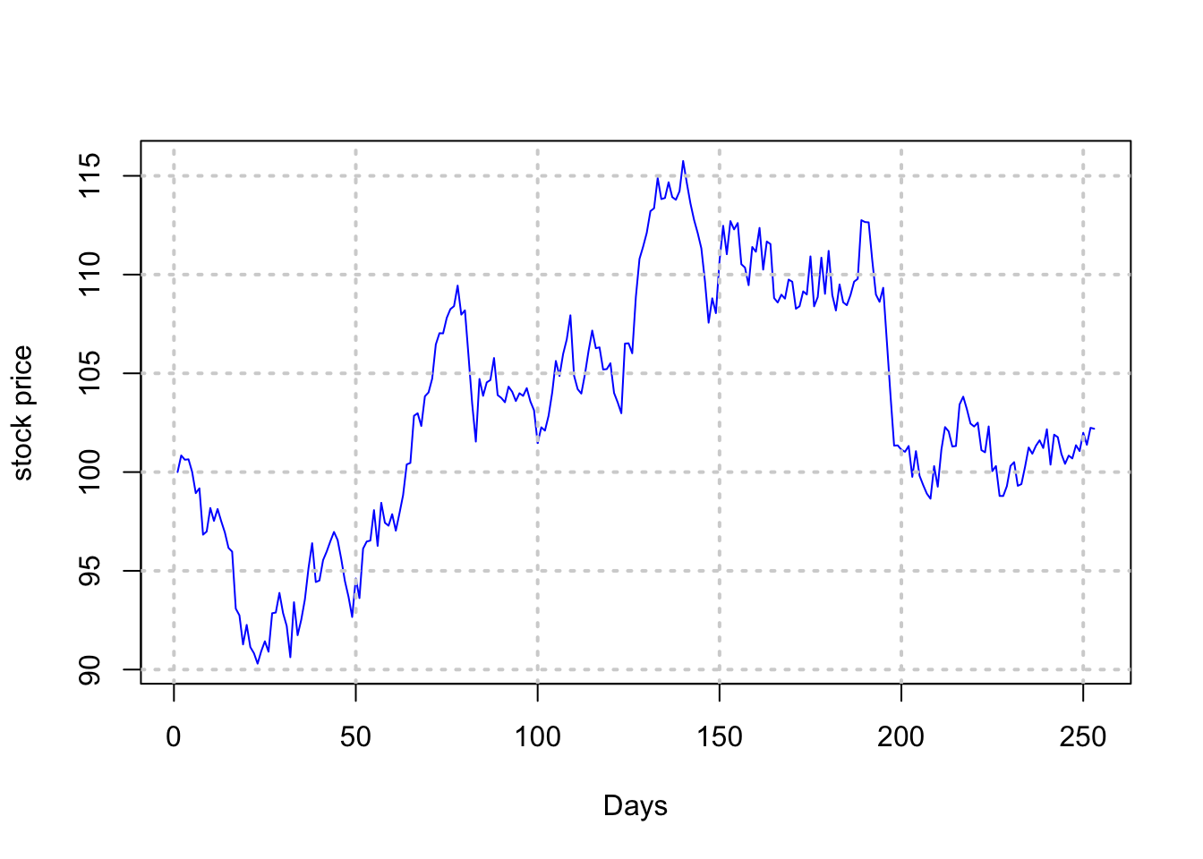
17.3 Vectorization
The same logic may be used to generate multiple paths of stock prices, in a vectorized way as follows. In the following example we generate 3 paths. Because of the vectorization, the run time does not increase linearly with the number of paths, and in fact, hardly increases at all.
s = matrix(0,3,n+1)
s[,1] = s0
for (j in seq(2,(n+1))) {
   s[,j]=s[,j-1]*exp((mu-sig^2/2)*h
    +sig*matrix(rnorm(3),3,1)*sqrt(h))
}
ymin = min(s); ymax = max(s)
plot(t(s)[,1],ylim=c(ymin,ymax),type="l",xlab="Days",ylab="stock price"); grid(lwd=2)
lines(t(s)[,2],col="red",lty=2)
lines(t(s)[,3],col="blue",lty=3)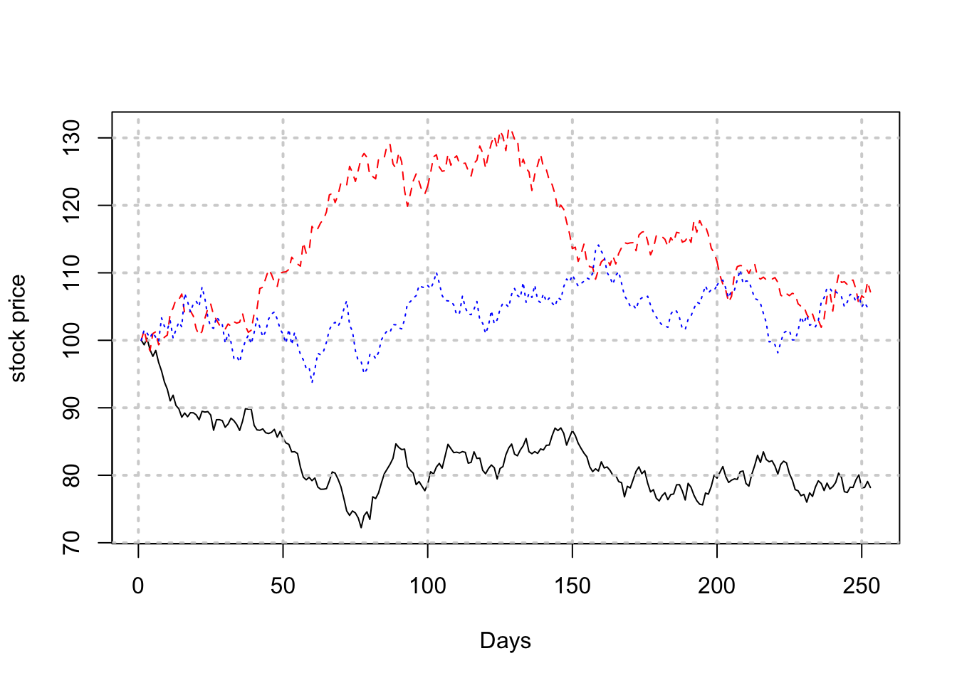
The plot code shows how to change the style of the path and its color.
If you generate many more paths, how can you find the probability of the stock ending up below a defined price? Can you do this directly from the discrete version of the Geometric Brownian motion process above?
17.4 Bivariate random variables
To convert two independent random variables \((e_1,e_2) \sim N(0,1)\) into two correlated random variables \((x_1,x_2)\) with correlation \(\rho\), use the following trannsformations. \[ x_1 = e_1, \quad \quad x_2 = \rho \cdot x_1 + \sqrt{1-\rho^2} \cdot x_2 \]
e = matrix(rnorm(20000),10000,2)
print(cor(e))
## [,1] [,2]
## [1,] 1.0000000000 0.0003501396
## [2,] 0.0003501396 1.0000000000print(cor(e[,1],e[,2]))## [1] 0.0003501396We see that these are uncorrelated random variables. Now we create a pair of correlated variates using the formula above.
rho = 0.6
x1 = e[,1]
x2 = rho*e[,1]+sqrt(1-rho^2)*e[,2]
cor(x1,x2)
## [1] 0.5941021Check algebraically that \(E[x_i]=0, i=1,2\), \(Var[x_i]=1, i=1,2\). Also check that \(Cov[x_1,x_2]=\rho = Corr[x_1,x_2]\).
print(mean(x1))## [1] -0.01568866print(mean(x2))## [1] 0.0004103859print(var(x1))## [1] 0.993663print(var(x2))## [1] 1.014452print(cov(x1,x2))## [1] 0.596480617.5 Multivariate random variables
These are generated using Cholesky decomposition. We may write a covariance matrix in decomposed form, i.e., \(\Sigma = L\; L'\), where \(L\) is a lower triangular matrix. Alternatively we might have an upper triangular decomposition, where \(U= L'\). Think of each component of the decomposition as a square-root of the covariance matrix.
#Original matrix
cv = matrix(c(0.01,0,0,0,0.04,0.02,0,0.02,0.16),3,3,byrow=TRUE)
print(cv)
## [,1] [,2] [,3]
## [1,] 0.01 0.00 0.00
## [2,] 0.00 0.04 0.02
## [3,] 0.00 0.02 0.16#Let's enhance it
cv[1,2]=0.005
cv[2,1]=0.005
cv[1,3]=0.005
cv[3,1]=0.005
print(cv)## [,1] [,2] [,3]
## [1,] 0.010 0.005 0.005
## [2,] 0.005 0.040 0.020
## [3,] 0.005 0.020 0.160We now compute the Cholesky decomposition of the covariance matrix.
L = t(chol(cv))
print(L)
## [,1] [,2] [,3]
## [1,] 0.10 0.00000000 0.0000000
## [2,] 0.05 0.19364917 0.0000000
## [3,] 0.05 0.09036961 0.3864367The Cholesky decomposition is now used to generate multivariate random variables with the correct correlation.
e = matrix(rnorm(3*10000),10000,3)
x = t(L %*% t(e))
print(dim(x))
## [1] 10000 3print(cov(x))## [,1] [,2] [,3]
## [1,] 0.009857043 0.004803601 0.005329556
## [2,] 0.004803601 0.040708872 0.021150791
## [3,] 0.005329556 0.021150791 0.161275573In the last calculation, we confirmed that the simulated data has the same covariance matrix as the one that we generated correlated random variables from.
17.6 Portfolio Computations
Let’s enter a sample mean vector and covariance matrix and then using some sample weights, we will perform some basic matrix computations for portfolios to illustrate the use of R.
mu = matrix(c(0.01,0.05,0.15),3,1)
cv = matrix(c(0.01,0,0,0,0.04,0.02,
                   0,0.02,0.16),3,3)
print(mu)
## [,1]
## [1,] 0.01
## [2,] 0.05
## [3,] 0.15print(cv)## [,1] [,2] [,3]
## [1,] 0.01 0.00 0.00
## [2,] 0.00 0.04 0.02
## [3,] 0.00 0.02 0.16w = matrix(c(0.3,0.3,0.4))
print(w)## [,1]
## [1,] 0.3
## [2,] 0.3
## [3,] 0.4The expected return of the portfolio is
muP = t(w) %*% mu
print(muP)
## [,1]
## [1,] 0.078And the standard deviation of the portfolio is
stdP = sqrt(t(w) %*% cv %*% w)
print(stdP)
## [,1]
## [1,] 0.1868154We thus generated the expected return and risk of the portfolio, i.e., the values \(0.078\) and \(0.187\), respectively.
We are interested in the risk of a portfolio, often measured by its variance. As we had seen in a previous chapter, as we increase \(n\), the number of securities in the portfolio, the variance keeps dropping, and asymptotes to a level equal to the average covariance of all the assets. It is interesting to see what happens as \(n\) increases through a very simple function in R that returns the standard deviation of the portfolio.
sigport = function(n,sig_i2,sig_ij) {
 cv = matrix(sig_ij,n,n)
 diag(cv) = sig_i2
 w = matrix(1/n,n,1)
 result = sqrt(t(w) %*% cv %*% w)
}
We now apply it to increasingly diversified portfolios.
n = seq(5,100,5)
risk_n = NULL
for (nn in n) {
 risk_n = c(risk_n,sigport(nn,0.04,0.01))
}
print(risk_n)
## [1] 0.1264911 0.1140175 0.1095445 0.1072381 0.1058301 0.1048809 0.1041976
## [8] 0.1036822 0.1032796 0.1029563 0.1026911 0.1024695 0.1022817 0.1021204
## [15] 0.1019804 0.1018577 0.1017494 0.1016530 0.1015667 0.1014889We can plot this to see the classic systematic risk plot. Systematic risk declines as the number of stocks in the portfolio increases.
plot(n,risk_n,type="l",ylab="Portfolio Std Dev")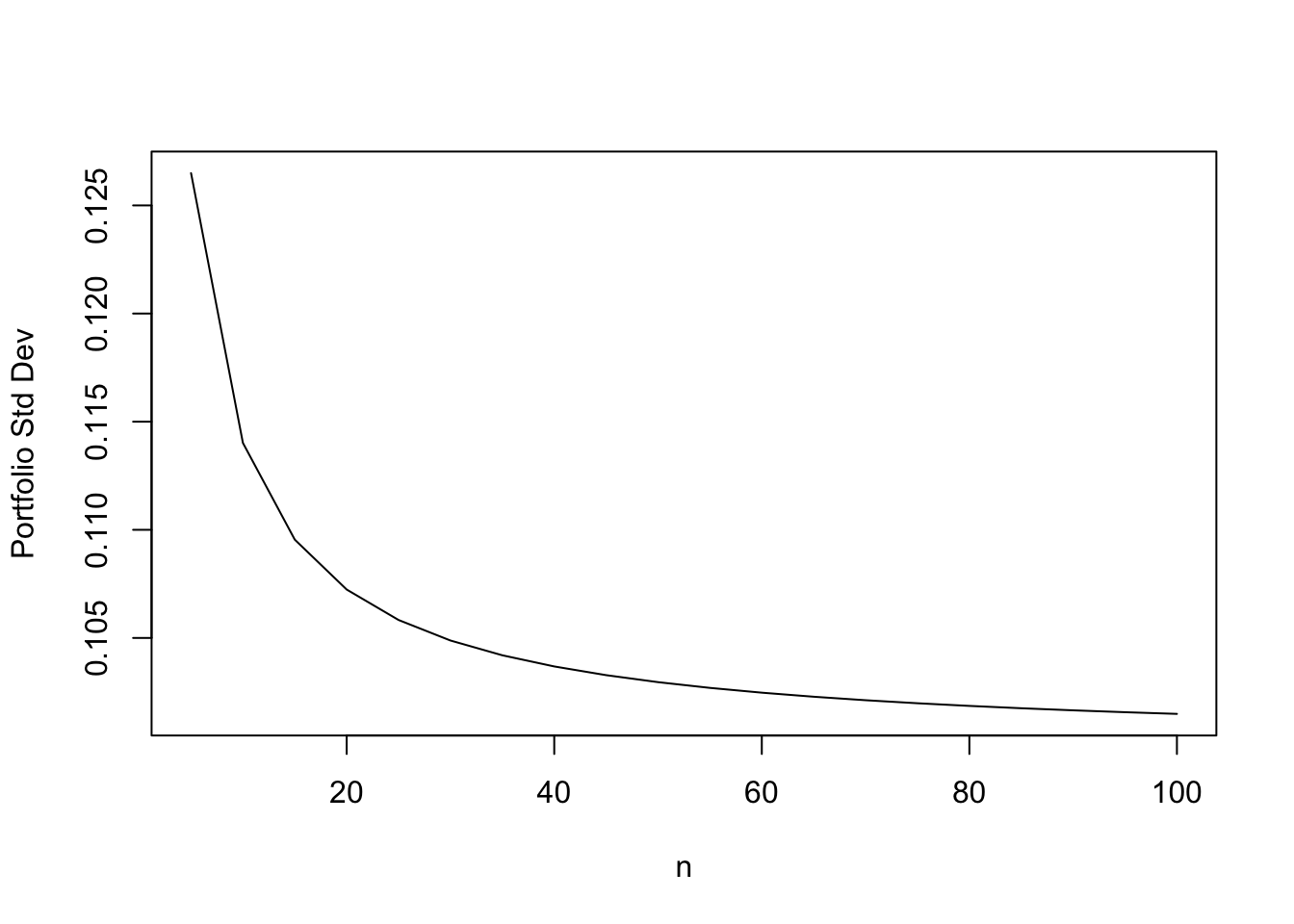
17.7 Optimal Portfolio
We will review the notation one more time. Assume that the risk free asset has return \(r_f\). And we have \(n\) risky assets, with mean returns \(\mu_i, i=1...n\). We need to invest in optimal weights \(w_i\) in each asset. Let \(w = [w_1, \ldots, w_n]'\) be a column vector of portfolio weights. We define \(\mu = [\mu_1, \ldots, \mu_n]'\) be the column vector of mean returns on each asset, and \({\bf 1} = [1,\ldots,1]'\) be a column vector of ones. Hence, the expected return on the portfolio will be
\[ E(R_p) = (1-w'{\bf 1}) r_f + w'\mu \]
The variance of return on the portfolio will be
\[ Var(R_p) = w' \Sigma w \]
where \(\Sigma\) is the covariance matrix of returns on the portfolio. The objective function is a trade-off between return and risk, with \(\beta\) modulating the balance between risk and return:
\[ U(R_p) = r_f + w'(\mu - r_f {\bf 1}) - \frac{\beta}{2} w'\Sigma w \]
The f.o.c. becomes a system of equations now (not a single equation), since we differentiate by an entire vector \(w\):
\[ \frac{dU}{dw'} = \mu - r_f {\bf 1} - \beta \Sigma w = {\bf 0} \]
where the RHS is a vector of zeros of dimension \(n\). Solving we have
\[ w = \frac{1}{\beta} \Sigma^{-1} (\mu - r_f {\bf 1}) \]
Therefore, allocation to the risky assets
- Increases when the relative return to it \((\mu - r_f {\bf 1})\) increases.
- Decreases when risk aversion increases.
- Decreases when riskiness of the assets increases as proxied for by \(\Sigma\).
n = 3
print(cv)
## [,1] [,2] [,3]
## [1,] 0.01 0.00 0.00
## [2,] 0.00 0.04 0.02
## [3,] 0.00 0.02 0.16print(mu)## [,1]
## [1,] 0.01
## [2,] 0.05
## [3,] 0.15rf=0.005
beta = 4
wuns = matrix(1,n,1)
print(wuns)## [,1]
## [1,] 1
## [2,] 1
## [3,] 1w = (1/beta)*(solve(cv) %*% (mu-rf*wuns))
print(w)## [,1]
## [1,] 0.1250000
## [2,] 0.1791667
## [3,] 0.2041667w_in_rf = 1-sum(w)
print(w_in_rf)## [1] 0.4916667What if we reduced beta?
beta = 3
w = (1/beta)*(solve(cv) %*% (mu-rf*wuns));
print(w)
## [,1]
## [1,] 0.1666667
## [2,] 0.2388889
## [3,] 0.2722222beta = 2
w = (1/beta)*(solve(cv) %*% (mu-rf*wuns));
print(w)## [,1]
## [1,] 0.2500000
## [2,] 0.3583333
## [3,] 0.4083333Notice that the weights in stocks scales linearly with \(\beta\). The relative proportions of the stocks themselves remains constant. Hence, \(\beta\) modulates the proportions invested in a risk-free asset and a stock portfolio, in which stock proportions remain same. It is as if the stock versus bond decision can be taken separately from the decision about the composition of the stock portfolio. This is known as the two-fund separation property, i.e., first determine the proportions in the bond fund vs stock fund and the allocation within each fund can be handled subsequently.