Chapter 16 Riding the Wave: Fourier Analysis
16.1 Introduction
Fourier analysis comprises many different connnections between infinite series, complex numbers, vector theory, and geometry. We may think of different applications: (a) fitting economic time series, (b) pricing options, (c) wavelets, (d) obtaining risk-neutral pricing distributions via Fourier inversion.
16.2 Fourier Series
16.2.1 Basic stuff
Fourier series are used to represent {} time series by combinations of sine and cosine waves. The time it takes for one cycle of the wave is called the period'' $T$ of the wave. Thefrequency’’ \(f\) of the wave is the number of cycles per second, hence,
\[ f = \frac{1}{T} \]
16.2.2 Unit Circle
We need some basic geometry on the unit circle.
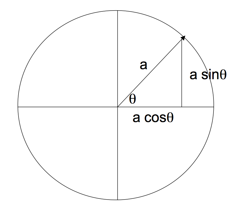
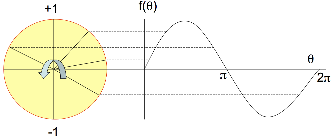
This circle is the unit circle if \(a=1\). There is a nice link between the unit circle and the sine wave. See the next figure for this relationship.
16.2.3 Angular velocity
Velocity is distance per time (in a given direction). For angular velocity we measure distance in degrees, i.e. degrees per unit of time. The usual symbol for angular velocity is \(\omega\). We can thus write
\[ \omega = \frac{\theta}{T}, \quad \theta = \omega T \]
Hence, we can state the function in equation (16.1) in terms of time as follows
\[ f(t) = a \sin \omega t \]
16.2.4 Fourier series
A Fourier series is a collection of sine and cosine waves, which when summed up, closely approximate any given waveform. We can express the Fourier series in terms of sine and cosine waves
\[ f(\theta) = a_0 + \sum_{n=1}^{\infty} \left( a_n \cos n\theta + b_n \sin n \theta \right) \]
\[ f(t) = a_0 + \sum_{n=1}^{\infty} \left( a_n \cos n\omega t + b_n \sin n \omega t \right) \]
The \(a_0\) is needed since the waves may not be symmetric around the x-axis.
16.2.5 Radians
Degrees are expressed in units of radians. A radian is an angle defined in the following figure.
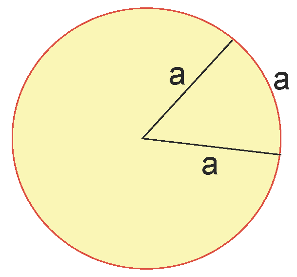
The angle here is a radian which is equal to 57.2958 degrees (approximately). This is slightly less than 60 degrees as you would expect to get with an equilateral triangle. Note that (since the circumference is \(2 \pi a\)) \(57.2958 \pi = 57.2958 \times 3.142 = 180\) degrees.
So now for the unit circle \[\begin{align} 2 \pi &= 360 \mbox{(degrees)}\\ \omega &= \frac{360}{T} \\ \omega &= \frac{2\pi}{T} \end{align}\] Hence, we may rewrite the Fourier series equation as: \[\begin{align} f(t) &= a_0 + \sum_{n=1}^{\infty} \left( a_n \cos n\omega t + b_n \sin n \omega t \right) \tag{16.2} \\ &= a_0 + \sum_{n=1}^{\infty} \left( a_n \cos \frac{2\pi n}{T} t + b_n \sin \frac{2\pi n}{T} t \right) \end{align}\]So we now need to figure out how to get the coefficients \(\{a_0,a_n,b_n\}\).
16.2.6 Solving for the coefficients
We start by noting the interesting phenomenon that sines and cosines are orthogonal, i.e. their inner product is zero. Hence, \[\begin{align} \int_0^T \sin(nt) . \cos(mt)\; dt &= 0, \forall n,m \\ \int_0^T \sin(nt) . \sin(mt)\; dt &= 0, \forall n \neq m \\ \int_0^T \cos(nt) . \cos(mt)\; dt &= 0, \forall n \neq m \end{align}\]What this means is that when we multiply one wave by another, and then integrate the resultant wave from \(0\) to \(T\) (i.e. over any cycle, so we could go from say \(-T/2\) to \(+T/2\) also), then we get zero, unless the two waves have the {} frequency. Hence, the way we get the coefficients of the Fourier series is as follows. Integrate both sides of the series in equation (16.2) from \(0\) to \(T\), i.e. \[ \int_0^T f(t) = \int_0^T a_0 \;dt + \int_0^T \left[\sum_{n=1}^{\infty} \left( a_n \cos n\omega t + b_n \sin n \omega t \right) \;dt \right] \] Except for the first term all the remaining terms are zero (integrating a sine or cosine wave over its cycle gives net zero). So we get \[ \int_0^T f(t) \;dt = a_0 T \] or \[ a_0 = \frac{1}{T} \int_0^T f(t) \;dt \]
Now lets try another integral, i.e. \[\begin{align} \int_0^T f(t) \cos(\omega t) &= \int_0^T a_0 \cos(\omega t) \;dt \\ & + \int_0^T \left[\sum_{n=1}^{\infty} \left( a_n \cos n\omega t + b_n \sin n \omega t \right)\cos(\omega t) \;dt \right] \end{align}\] Here, all terms are zero except for the term in \(a_1 \cos(\omega t)\cos(\omega t)\), because we are multiplying two waves (pointwise) that have the same frequency. So we get \[\begin{align} \int_0^T f(t) \cos(\omega t) &= \int_0^T a_1 \cos(\omega t)\cos(\omega t) \;dt \\ &= a_1 \; \frac{T}{2} \end{align}\]How? Note here that for unit amplitude, integrating \(\cos(\omega t)\) over one cycle will give zero. If we multiply \(\cos(\omega t)\) by itself, we flip all the wave segments from below to above the zero line. The product wave now fills out half the area from \(0\) to \(T\), so we get \(T/2\). Thus \[ a_1 = \frac{2}{T} \int_0^T f(t) \cos(\omega t) \] We can get all \(a_n\) this way - just multiply by \(\cos(n \omega t)\) and integrate. We can also get all \(b_n\) this way - just multiply by \(\sin(n \omega t)\) and integrate.
This forms the basis of the following summary results that give the coefficients of the Fourier series. \[\begin{align} a_0 &= \frac{1}{T} \int_{-T/2}^{T/2} f(t) \;dt = \frac{1}{T} \int_{0}^{T} f(t) \;dt\\ a_n &= \frac{1}{T/2} \int_{-T/2}^{T/2} f(t) \cos(n\omega t)\;dt = \frac{2}{T} \int_{0}^{T} f(t) \cos(n\omega t)\;dt \\ b_n &= \frac{1}{T/2} \int_{-T/2}^{T/2} f(t) \sin(n\omega t)\;dt = \frac{2}{T} \int_{0}^{T} f(t) \sin(n\omega t)\;dt \end{align}\]16.3 Complex Algebra
Just for fun, recall that \[ e = \sum_{n=0}^{\infty} \frac{1}{n!}. \] and \[ e^{i \theta} = \sum_{n=0}^{\infty} \frac{1}{n!} (i \theta)^n \] \[\begin{align} \cos(\theta) &= 1 + 0.\theta - \frac{1}{2!} \theta^2 + 0.\theta^3 + \frac{1}{4!} \theta^2 + \ldots \\ i \sin(\theta) &= 0 + i \theta + 0.\theta^2 - \frac{1}{3!}i\theta^3 + 0.\theta^4 + \ldots \end{align}\] Which leads into the famous Euler’s formula: \[\begin{equation} \tag{16.3} e^{i \theta} = \cos \theta + i \sin \theta \end{equation}\] and the corresponding \[\begin{equation} \tag{16.4} e^{-i \theta} = \cos \theta - i \sin \theta \end{equation}\]Recall also that \(\cos(-\theta) = \cos(\theta)\). And \(\sin(-\theta) = - \sin(\theta)\). Note also that if \(\theta = \pi\), then \[ e^{-i \pi} = \cos(\pi) - i \sin(\pi) = -1 + 0 \] which can be written as \[ e^{-i \pi} + 1 = 0 \] an equation that contains five fundamental mathematical constants: \(\{i, \pi, e, 0, 1\}\), and three operators \(\{+, -, =\}\).
16.3.1 Trig to Complex
Using equations (16.3) and (16.4) gives \[\begin{align} \cos \theta &= \frac{1}{2} (e^{i \theta} + e^{-i \theta}) \\ \sin \theta &= \frac{1}{2}i (e^{i \theta} - e^{-i \theta}) \end{align}\] Now, return to the Fourier series, \[\begin{align} f(t) &= a_0 + \sum_{n=1}^{\infty} \left( a_n \cos n\omega t + b_n \sin n \omega t \right) \\ &= a_0 + \sum_{n=1}^{\infty} \left( a_n \frac{1}{2} (e^{in\omega t}+e^{-in\omega t}) + b_n \frac{1}{2i} (e^{in\omega t} - e^{-i n \omega t}) \right) \\ &= a_0 + \sum_{n=1}^{\infty} \left( A_n e^{in\omega t} + B_n e^{-in \omega t} \right)\\ & \mbox{where} \nonumber \\ & A_n = \frac{1}{T} \int_0^T f(t) e^{-in\omega t} \;dt \nonumber \\ & B_n = \frac{1}{T} \int_0^T f(t) e^{in\omega t} \;dt \nonumber \end{align}\]How? Start with
\[ f(t) = a_0 + \sum_{n=1}^{\infty} \left( a_n \frac{1}{2} (e^{in\omega t}+e^{-in\omega t}) + b_n \frac{1}{2i} (e^{in\omega t} - e^{-i n \omega t}) \right) \]
Then
\[ f(t) = a_0 + \sum_{n=1}^{\infty} \left( a_n \frac{1}{2} (e^{in\omega t}+e^{-in\omega t}) + b_n \frac{i}{2i^2} (e^{in\omega t} - e^{-i n \omega t}) \right) \]
\[ = a_0 + \sum_{n=1}^{\infty} \left( a_n \frac{1}{2} (e^{in\omega t}+e^{-in\omega t}) + b_n \frac{i}{-2} (e^{in\omega t} - e^{-i n \omega t}) \right) \]
\[\begin{equation} f(t) = a_0 + \sum_{n=1}^{\infty} \left( \frac{1}{2}(a_n -ib_n)e^{in\omega t} + \frac{1}{2}(a_n + ib_n)e^{-in\omega t} \right) \tag{16.5} \end{equation}\] Note that from equations (16.3) and (16.4), \[\begin{align} a_n &= \frac{2}{T} \int_0^T f(t) \cos(n \omega t) \;dt \\ &= \frac{2}{T} \int_0^T f(t) \frac{1}{2} [e^{in\omega t} + e^{-in\omega t}] \;dt \\ a_n &= \frac{1}{T} \int_0^T f(t) [e^{in\omega t} + e^{-in\omega t}] \;dt \tag{16.6} \end{align}\] In the same way, we can handle \(b_n\), to get \[\begin{align} b_n &= \frac{2}{T} \int_0^T f(t) \sin(n \omega t) \;dt \\ &= \frac{2}{T} \int_0^T f(t) \frac{1}{2i} [e^{in\omega t} - e^{-in\omega t}] \;dt \\ &= \frac{1}{i}\frac{1}{T} \int_0^T f(t) [e^{in\omega t} - e^{-in\omega t}] \;dt \end{align}\] So that \[\begin{equation} i b_n = \frac{1}{T} \int_0^T f(t) [e^{in\omega t} - e^{-in\omega t}] \;dt \tag{16.7} \end{equation}\] So from equations (16.6) and (16.7), we get \[\begin{align} \frac{1}{2}(a_n - i b_n) &= \frac{1}{T} \int_0^T f(t) e^{-in\omega t} \;dt \equiv A_n\\ \frac{1}{2}(a_n + i b_n) &= \frac{1}{T} \int_0^T f(t) e^{in\omega t} \;dt \equiv B_n \end{align}\] Put these back into equation (16.5) to get \[\begin{align} f(t) &= a_0 + \sum_{n=1}^{\infty} \left( \frac{1}{2}(a_n -ib_n)e^{in\omega t} + \frac{1}{2}(a_n + ib_n)e^{-in\omega t} \right) \\ &= a_0 + \sum_{n=1}^{\infty} \left( A_n e^{in\omega t} + B_n e^{-in \omega t} \right) \end{align}\]16.3.2 Getting rid of \(a_0\)
Note that if we expand the range of the first summation to start from \(n=0\), then we have a term \(A_0 e^{i0 \omega t} = A_0 \equiv a_0\). So we can then write our expression as \[ f(t) = \sum_{n=0}^{\infty} A_n e^{in\omega t} + \sum_{n=1}^{\infty} B_n e^{-in \omega t} \mbox{ (sum of A runs from zero)} \]
16.3.3 Collapsing and Simplifying
So now we want to collapse these two terms together. Lets note that \[ \sum_{n=1}^2 x^n = x^1 + x^2 = \sum_{n=-2}^{-1} x^{-n} = x^2 + x^1 \] Applying this idea, we get \[\begin{align} f(t) &= \sum_{n=0}^{\infty} A_n e^{in\omega t} + \sum_{n=1}^{\infty} B_n e^{-in \omega t} \\ &= \sum_{n=0}^{\infty} A_n e^{in\omega t} + \sum_{n=-\infty}^{-1} B_{(-n)} e^{in \omega t} \\ & \mbox{where} \nonumber \\ & B_{(-n)} = \frac{1}{T} \int_0^T f(t) e^{-in\omega t} \;dt \nonumber = A_n \\ &= \sum_{n=-\infty}^{\infty} C_n e^{in\omega t}\\ & \mbox{where} \nonumber \\ & C_n = \frac{1}{T} \int_0^T f(t) e^{-in\omega t} \;dt \nonumber \end{align}\]where we just renamed \(A_n\) to \(C_n\) for clarity. The big win here is that we have been able to subsume \(\{a_0,a_n,b_n\}\) all into one coefficient set \(C_n\). For completeness we write \[ f(t) = a_0 + \sum_{n=1}^{\infty} \left( a_n \cos n\omega t + b_n \sin n \omega t \right) =\sum_{n=-\infty}^{\infty} C_n e^{in\omega t} \] This is the complex number representation of the Fourier series.
16.4 Fourier Transform
The FT is a cool technique that allows us to go from the Fourier series, which needs a period \(T\) to waves that are aperiodic. The idea is to simply let the period go to infinity. Which means the frequency gets very small. We can then sample a slice of the wave to do analysis.
We will replace \(f(t)\) with \(g(t)\) because we now need to use \(f\) or \(\Delta f\) to denote frequency. Recall that \[ \omega = \frac{2\pi}{T} = 2\pi f, \quad n\omega = 2 \pi f_n \] To recap \[\begin{align} g(t) &= \sum_{n=-\infty}^{\infty} C_n e^{in\omega t} = \sum_{n=-\infty}^{\infty} C_n e^{i 2\pi f t}\\ C_n &= \frac{1}{T} \int_0^T g(t) e^{-in\omega t} \;dt \end{align}\] This may be written alternatively in frequency terms as follows \[ C_n = \Delta f \int_{-T/2}^{T/2} g(t) e^{-i 2\pi f_n t} \;dt \] which we substitute into the formula for \(g(t)\) and get \[ g(t) = \sum_{n=-\infty}^{\infty} \left[\Delta f \int_{-T/2}^{T/2} g(t) e^{-i 2\pi f_n t} \;dt \right]e^{in\omega t} \] Taking limits \[ g(t) = \lim_{T \rightarrow \infty} \sum_{n=-\infty}^{\infty} \left[\int_{-T/2}^{T/2} g(t) e^{-i 2\pi f_n t} \;dt \right]e^{i 2 \pi f_n t} \Delta f \] gives a double integral \[ g(t) = \int_{-\infty}^{\infty} \underbrace{\left[\int_{-\infty}^{\infty} g(t) e^{-i 2\pi f t} \;dt \right]}_{G(f)} e^{i 2 \pi f t} \;df \] The \(dt\) is for the time domain and the \(df\) for the frequency domain. Hence, the {} goes from the time domain into the frequency domain, given by \[ G(f) = \int_{-\infty}^{\infty} g(t) e^{-i 2\pi f t} \;dt \] The {} goes from the frequency domain into the time domain \[ g(t) = \int_{-\infty}^{\infty} G(f) e^{i 2 \pi f t} \;df \] And the {} are as before \[ C_n = \frac{1}{T} \int_0^T g(t) e^{-i 2\pi f_n t} \;dt = \frac{1}{T} \int_0^T g(t) e^{-in\omega t} \; dt \] Notice the incredible similarity between the coefficients and the transform. Note the following:The spectrum of a wave is a graph showing its component frequencies, i.e. the quantity in which they occur. It is the frequency components of the waves. But it does not give their amplitudes.
16.4.1 Empirical Example
We can use the Fourier transform function in R to compute the main component frequencies of the times series of interest rate data as follows:
library(zoo)##
## Attaching package: 'zoo'## The following objects are masked from 'package:base':
##
## as.Date, as.Date.numericrd = read.table("DSTMAA_data/tryrates.txt",header=TRUE)
r1 = rd$FYGT1
dt = as.yearmon(rd$DATE,"%b-%y")
plot(dt,r1,type="l",ylab="One-Year Rate")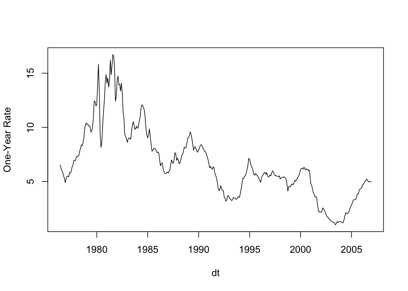
The line with
dr1 = resid(lm(r1 ~ seq(along = r1)))detrends the series, and when we plot it we see that its done. We can then subject the detrended line to fourier analysis. The plot of the fit of the detrended one-year interest rates is here:
dr1 = resid(lm(r1 ~ seq(along = r1)))
plot(dt,dr1,type="l",ylab="Detrended 1y Rate")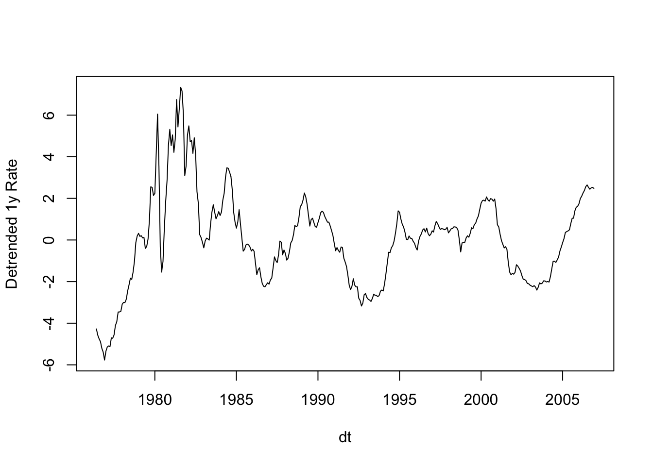
Now, carry out the Fourier transform.
y=fft(dr1)
plot(abs(y),type="l")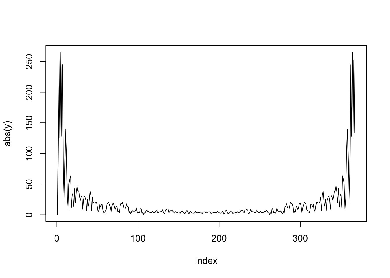
Its easy to see that the series has short frequencies and long frequencies. Essentially there are two factors. If we do a factor analysis of interest rates, it turns out we get two factors as well. See Chapter @ref{DiscriminantFactorAnalysis}.
16.5 Application to Binomial Option Pricing
To implement the option pricing in Cerny (2009), Chapter 7, Figure 8.
ifft = function(x) { fft(x,inverse=TRUE)/length(x) }
ct = c(599.64,102,0,0)
q = c(0.43523,0.56477,0,0)
R = 1.0033
ifft(fft(ct)*( (4*ifft(q)/R)^3) )
## [1] 81.36464+0i 115.28447+0i 265.46949+0i 232.62076+0iThe resulting price is 81.36.
16.6 Application to probability functions
16.6.1 Characteristic functions
A characteristic function of a variable \(x\) is given by the expectation of the following function of \(x\): \[ \phi(s) = E[e^{isx}] = \int_{-\infty}^{\infty} e^{isx} f(x) \; dx \] where \(f(x)\) is the probability density of \(x\). By Taylor series for \(e^{isx}\) we have \[\begin{align} \int_{-\infty}^{\infty} e^{isx} f(x) \; dx &= \int_{-\infty}^{\infty} [1+isx + \frac{1}{2} (isx)^2 + \ldots] f(x)dx \\ &= \sum_{j=0}^{\infty} \frac{(is)^j}{j!} m_j \\ &= 1 + (is) m_1 + \frac{1}{2} (is)^2 m_2 + \frac{1}{6} (is)^3 m_3 + \ldots \end{align}\]where \(m_j\) is the \(j\)-th moment.
It is therefore easy to see that \[ m_j = \frac{1}{i^j} \left[\frac{d\phi(s)}{ds} \right]_{s=0} \] where \(i=\sqrt{-1}\).
16.6.2 Finance application
In a paper in 1993, Steve Heston developed a new approach to valuing stock and foreign currency options using a Fourier inversion technique. See also Duffie, Pan and Singleton (2001) for extension to jumps, and Chacko and Das (2002) for a generalization of this to interest-rate derivatives with jumps.
Lets explore a much simpler model of the same so as to get the idea of how we can get at probability functions if we are given a stochastic process for any security. When we are thinking of a dynamically moving financial variable (say \(x_t\)), we are usually interested in knowing what the probability is of this variable reaching a value \(x_{\tau}\) at time \(t=\tau\), given that right now, it has value \(x_0\) at time \(t=0\). Note that \(\tau\) is the remaining time to maturity.
Suppose we have the following financial variable \(x_t\) following a very simple Brownian motion, i.e. \[
dx_t = \mu \; dt + \sigma\; dz_t
\] Here, \(\mu\) is known as its drift" andsigma’’ is the volatility. The differential equation above gives the movement of the variable \(x\) and the term \(dz\) is a Brownian motion, and is a random variable with normal distribution of mean zero, and variance \(dt\).
What we are interested in is the characteristic function of this process. The characteristic function of \(x\) is defined as the Fourier transform of \(x\), i.e. \[ F(x) = E[e^{isx}] = \int e^{isx} f(x) ds \] where \(s\) is the Fourier variable of integration, and \(i=\sqrt{-1}\), as usual. Notice the similarity to the Fourier transforms described earlier in the note. It turns out that once we have the characteristic function, then we can obtain by simple calculations the probability function for \(x\), as well as all the moments of \(x\).
16.6.3 Solving for the characteristic function
We write the characteristic function as \(F(x,\tau; s)\). Then, using Ito’s lemma we have \[ dF = F_x dx + \frac{1}{2} F_{xx} (dx)^2 -F_{\tau} dt \] \(F_x\) is the first derivative of \(F\) with respect to \(x\); \(F_{xx}\) is the second derivative, and \(F_{\tau}\) is the derivative with respect to remaining maturity. Since \(F\) is a characteristic (probability) function, the expected change in \(F\) is zero. \[ E(dF) = \mu F_x \;dt+ \frac{1}{2} \sigma^2 F_{xx} \; dt- F_{\tau}\; dt = 0 \] which gives a PDE in \((x,\tau)\): \[ \mu F_x + \frac{1}{2} \sigma^2 F_{xx} - F_{\tau} = 0 \] We need a boundary condition for the characteristic function which is \[ F(x,\tau=0;s) = e^{isx} \] We solve the PDE by making an educated guess, which is \[ F(x,\tau;s) = e^{isx + A(\tau)} \] which implies that when \(\tau=0\), \(A(\tau=0)=0\) as well. We can see that \[\begin{align} F_x &= isF \\ F_{xx} &= -s^2 F\\ F_{\tau} &= A_{\tau} F \end{align}\] Substituting this back in the PDE gives \[\begin{align} \mu is F - \frac{1}{2} \sigma^2 s^2 F - A_{\tau} F &= 0 \\ \mu is - \frac{1}{2} \sigma^2 s^2 - A_{\tau} &= 0 \\ \frac{dA}{d\tau} &= \mu is - \frac{1}{2} \sigma^2 s^2 \\ \mbox{gives: } A(\tau) &= \mu is \tau - \frac{1}{2} \sigma^2 s^2 \tau, \quad \mbox{because } A(0)=0 \end{align}\]Thus we finally have the characteristic function which is \[ F(x,\tau; s) = \exp[isx + \mu is \tau -\frac{1}{2} \sigma^2 s^2 \tau] \]
16.6.4 Computing the moments
In general, the moments are derived by differentiating the characteristic function y \(s\) and setting \(s=0\). The \(k\)-th moment will be \[ E[x^k] = \frac{1}{i^k} \left[ \frac{\partial^k F}{\partial s^k} \right]_{s=0} \] Lets test it by computing the mean (\(k=1\)): \[ E(x) = \frac{1}{i} \left[ \frac{\partial F}{\partial s} \right]_{s=0} = x + \mu \tau \] where \(x\) is the current value \(x_0\). How about the second moment? \[ E(x^2) = \frac{1}{i^2} \left[ \frac{\partial^2 F}{\partial s^2} \right]_{s=0} =\sigma^2 \tau + (x+\mu \tau)^2 = \sigma^2 \tau + E(x)^2 \] Hence, the variance will be \[ Var(x) = E(x^2) - E(x)^2 = \sigma^2 \tau + E(x)^2 - E(x^2) = \sigma^2 \tau \]
16.6.5 Probability density function
It turns out that we can ``invert’’ the characteristic function to get the pdf (boy, this characteristic function sure is useful!). Again we use Fourier inversion, which result is stated as follows: \[ f(x_{\tau} | x_0) = \frac{1}{\pi} \int_0^{\infty} Re[e^{-isx_{\tau}}] F(x_0,\tau; s)\; ds \]
Here is an implementation
#Model for fourier inversion for arithmetic brownian motion

x0 = 10
mu = 10
sig = 5
tau = 0.25
s = (0:10000)/100
ds = s[2]-s[1]

phi =  exp(1i*s*x0+mu*1i*s*tau-0.5*s^2*sig^2*tau)

x = (0:250)/10
fx=NULL
for (k in 1:length(x)) {
  g = sum(Re(exp(-1i*s*x[k]) * phi * ds))/pi
  #print(c(x[k],g))
  fx = c(fx,g)
}

plot(x,fx,type="l",main="Inverse Fourier plot")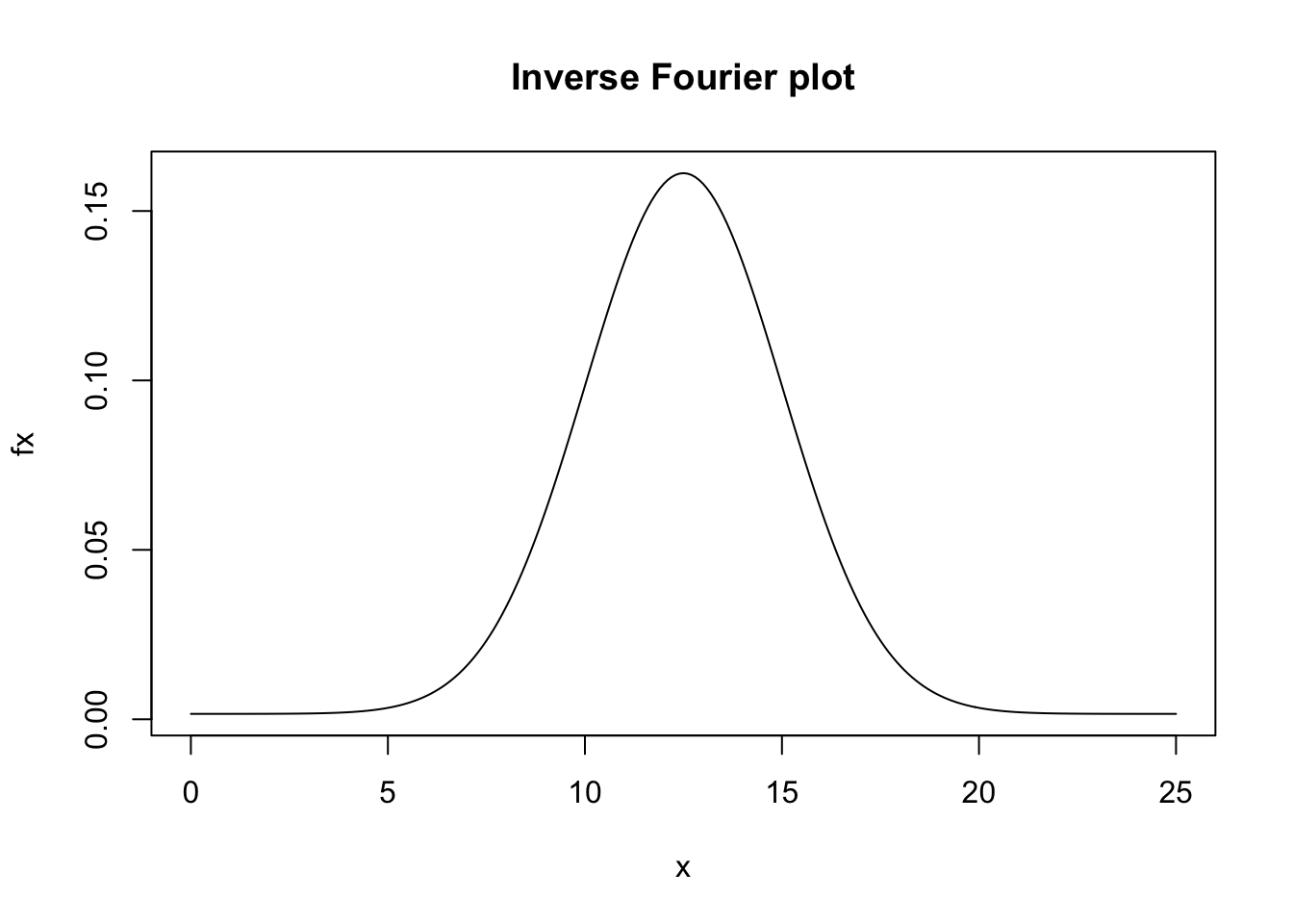
References
Cerny, Ales. 2009. Mathematical Techniques in Finance: Tools for Incomplete Markets. Princeton, New Jersey: Princeton University Press.