Chapter 15 Product Market Forecasting using the Bass Model
15.1 Main Ideas
The Bass product diffusion model is a classic one in the marketing literature. It has been successfully used to predict the market shares of various newly introduced products, as well as mature ones.
The main idea of the model is that the adoption rate of a product comes from two sources:
The propensity of consumers to adopt the product independent of social influences to do so.
The additional propensity to adopt the product because others have adopted it. Hence, at some point in the life cycle of a good product, social contagion, i.e. the influence of the early adopters becomes sufficiently strong so as to drive many others to adopt the product as well. It may be going too far to think of this as a network effect, because Frank Bass did this work well before the concept of network effect was introduced, but essentially that is what it is.
The Bass model shows how the information of the first few periods of sales data may be used to develop a fairly good forecast of future sales. One can easily see that whereas this model came from the domain of marketing, it may just as easily be used to model forecasts of cashflows to determine the value of a start-up company.
15.2 Historical Examples
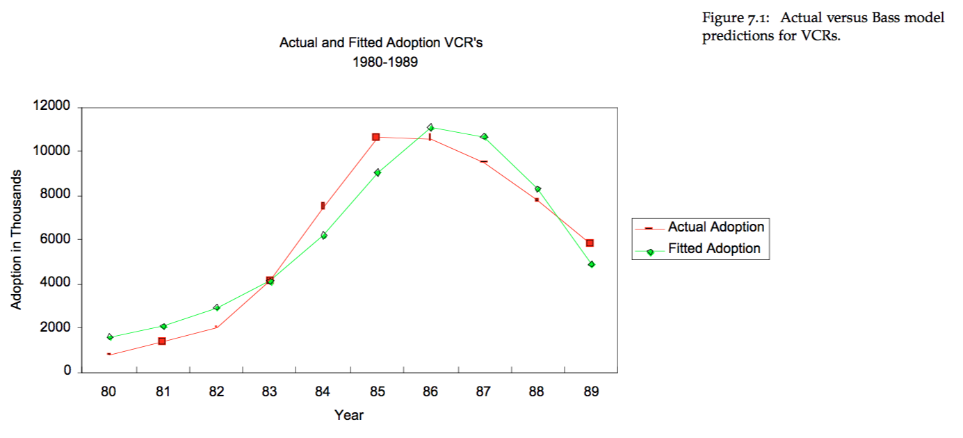
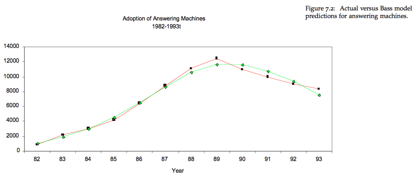
There are some classic examples from the literature of the Bass model providing a very good forecast of the ramp up in product adoption as a function of the two sources described above. See for example the actual versus predicted market growth for VCRs in the 80s and the adoption of answering machines shown in the Figures below.
15.3 The Basic Idea
We follow the exposition in Bass (1969).
Define the cumulative probability of purchase of a product from time zero to time \(t\) by a single individual as \(F(t)\). Then, the probability of purchase at time \(t\) is the density function \(f(t) = F'(t)\).
The rate of purchase at time \(t\), given no purchase so far, logically follows, i.e.
\[ \frac{f(t)}{1-F(t)}. \]
Modeling this is just like modeling the adoption rate of the product at a given time \(t\).
15.4 Main Differential Equation
Bass suggested that this adoption rate be defined as
\[ \frac{f(t)}{1-F(t)} = p + q\; F(t). \]
where we may think of \(p\) as defining the independent rate of a consumer adopting the product, and \(q\) as the imitation rate, because it modulates the impact from the cumulative intensity of adoption, \(F(t)\).
Hence, if we can find \(p\) and \(q\) for a product, we can forecast its adoption over time, and thereby generate a time path of sales. To summarize:
- \(p\): coefficient of innovation.
- \(q\): coefficient of imitation.
15.5 Solving the Model for \(F(t)\)
We rewrite the Bass equation:
\[ \frac{dF/dt}{1-F} = p + q\; F. \]
and note that \(F(0)=0\).
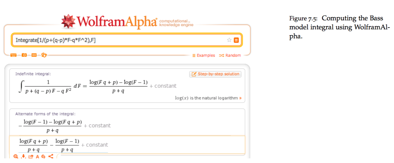
The steps in the solution are: \[ \begin{eqnarray} \frac{dF}{dt} &=& (p+qF)(1-F) \\ \frac{dF}{dt} &=& p + (q-p)F - qF^2 \\ \int \frac{1}{p + (q-p)F - qF^2}\;dF &=& \int dt \\ \frac{\ln(p+qF) - \ln(1-F)}{p+q} &=& t+c_1 \quad \quad (*) \\ t=0 &\Rightarrow& F(0)=0 \\ t=0 &\Rightarrow& c_1 = \frac{\ln p}{p+q} \\ F(t) &=& \frac{p(e^{(p+q)t}-1)}{p e^{(p+q)t} + q} \end{eqnarray} \]
15.6 Another solution
An alternative approach (this was suggested by students Muhammad Sagarwalla based on ideas from Alexey Orlovsky) goes as follows. First, split the integral above into partial fractions.
\[ \int \frac{1}{(p+qF)(1-F)}\;dF = \int dt \]
So we write \[ \begin{eqnarray} \frac{1}{(p+qF)(1-F)} &=& \frac{A}{p+qF} + \frac{B}{1-F}\\ &=& \frac{A-AF+pB+qFB}{(p+qF)(1-F)}\\ &=& \frac{A+pB+F(qB-A)}{(p+qF)(1-F)} \end{eqnarray} \]
This implies that \[ \begin{eqnarray} A+pB &=& 1 \\ qB-A &=& 0 \end{eqnarray} \]
Solving we get \[ \begin{eqnarray} A &=& q/(p+q)\\ B &=& 1/(p+q) \end{eqnarray} \]
so that \[ \begin{eqnarray} \int \frac{1}{(p+qF)(1-F)}\;dF &=& \int dt \\ \int \left(\frac{A}{p+qF} + \frac{B}{1-F}\right) \; dF&=& t + c_1 \\ \int \left(\frac{q/(p+q)}{p+qF} + \frac{1/(p+q)}{1-F}\right) \; dF&=& t+c_1\\ \frac{1}{p+q}\ln(p+qF) - \frac{1}{p+q}\ln(1-F) &=& t+c_1\\ \frac{\ln(p+qF) - \ln(1-F)}{p+q} &=& t+c_1 \end{eqnarray} \]
which is the same as equation (*). The solution as before is
\[ F(t) = \frac{p(e^{(p+q)t}-1)}{p e^{(p+q)t} + q} \]
15.7 Solve for \(f(t)\)
We may also solve for
\[ f(t) = \frac{dF}{dt} = \frac{e^{(p+q)t}\; p \; (p+q)^2}{[p e^{(p+q)t} + q]^2} \]
Therefore, if the target market is of size \(m\), then at each \(t\), the adoptions are simply given by \(m \times f(t)\).
15.8 Example
For example, set \(m=100,000\), \(p=0.01\) and \(q=0.2\). Then the adoption rate is shown in the Figure below.
f = function(p,q,t) {
    res = (exp((p+q)*t)*p*(p+q)^2)/(p*exp((p+q)*t)+q)^2
}
t = seq(1,20)
m = 100000
p = 0.01
q = 0.20
plot(t,m*f(p,q,t),type="l",col="blue",lwd=3,xlab="Time (years)",ylab="Adoptions")
grid(lwd=2)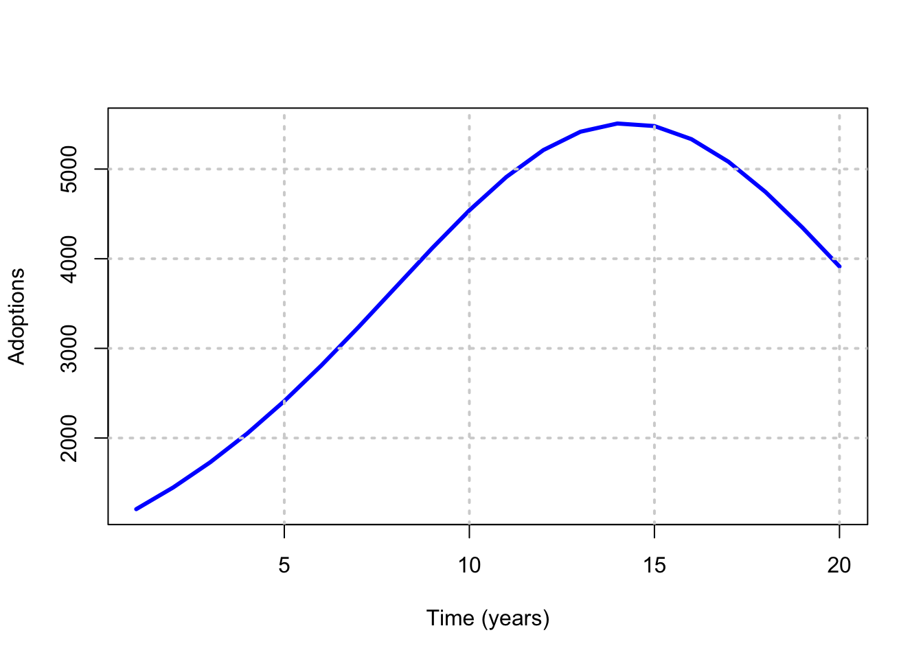
15.9 Symbolic Math in R
#BASS MODEL
FF = expression(p*(exp((p+q)*t)-1)/(p*exp((p+q)*t)+q))
print(FF)
## expression(p * (exp((p + q) * t) - 1)/(p * exp((p + q) * t) +
## q))#Take derivative
ff = D(FF,"t")
print(ff)## p * (exp((p + q) * t) * (p + q))/(p * exp((p + q) * t) + q) -
## p * (exp((p + q) * t) - 1) * (p * (exp((p + q) * t) * (p +
## q)))/(p * exp((p + q) * t) + q)^2#SET UP THE FUNCTION
ff = function(p,q,t) {
res = D(FF,"t")
}#NOTE THE USE OF eval
m=100000; p=0.01; q=0.20; t=seq(1,20)
plot(t,m*eval(ff(p,q,t)),type="l",col="red",lwd=3)
grid(lwd=2)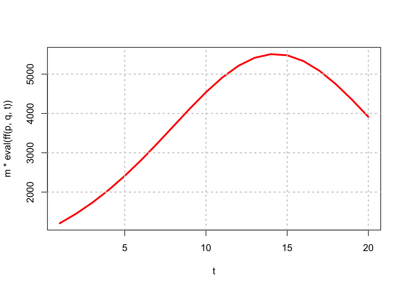
15.11 Calibration
How do we get coefficients \(p\) and \(q\)? Given we have the current sales history of the product, we can use it to fit the adoption curve.
- Sales in any period are: \(s(t) = m \; f(t)\).
- Cumulative sales up to time \(t\) are: \(S(t) = m \; F(t)\).
Substituting for \(f(t)\) and \(F(t)\) in the Bass equation gives:
\[ \frac{s(t)/m}{1-S(t)/m} = p + q\; S(t)/m \]
We may rewrite this as
\[ s(t) = [p+q\; S(t)/m][m - S(t)] \]
Therefore, \[ \begin{eqnarray} s(t) &=& \beta_0 + \beta_1 \; S(t) + \beta_2 \; S(t)^2 \quad (BASS) \\ \beta_0 &=& pm \\ \beta_1 &=& q-p \\ \beta_2 &=& -q/m \end{eqnarray} \]
Equation (BASS) may be estimated by a regression of sales against cumulative sales. Once the coefficients in the regression \(\{\beta_0, \beta_1, \beta_2\}\) are obtained, the equations above may be inverted to determine the values of \(\{m,p,q\}\). We note that since
\[ \beta_1 = q-p = -m \beta_2 - \frac{\beta_0}{m}, \]
we obtain a quadratic equation in \(m\):
\[ \beta_2 m^2 + \beta_1 m + \beta_0 = 0 \]
Solving we have
\[ m = \frac{-\beta_1 \pm \sqrt{\beta_1^2 - 4 \beta_0 \beta_2}}{2 \beta_1} \]
and then this value of \(m\) may be used to solve for
\[ p = \frac{\beta_0}{m}; \quad \quad q = - m \beta_2 \]
15.12 iPhone Sales Forecast
As an example, let’s look at the trend for iPhone sales (we store the quarterly sales in a file and read it in, and then undertake the Bass model analysis). We get the data from: http://www.statista.com/statistics/263401/global-apple-iphone-sales-since-3rd-quarter-2007/
The R code for this computation is as follows:
#USING APPLE iPHONE SALES DATA
data = read.table("DSTMAA_data/iphone_sales.txt",header=TRUE)
print(head(data))
## Quarter Sales_MM_units
## 1 Q3_07 0.27
## 2 Q4_07 1.12
## 3 Q1_08 2.32
## 4 Q2_08 1.70
## 5 Q3_08 0.72
## 6 Q4_08 6.89print(tail(data))## Quarter Sales_MM_units
## 30 Q4_14 39.27
## 31 Q1_15 74.47
## 32 Q2_15 61.17
## 33 Q3_15 47.53
## 34 Q4_15 48.05
## 35 Q1_16 74.78#data = data[1:31,]
data = data[1:length(data[,1]),]isales = data[,2]
cum_isales = cumsum(isales)
cum_isales2 = cum_isales^2
res = lm(isales ~ cum_isales+cum_isales2)
print(summary(res))##
## Call:
## lm(formula = isales ~ cum_isales + cum_isales2)
##
## Residuals:
## Min 1Q Median 3Q Max
## -14.050 -3.413 -1.429 2.905 19.987
##
## Coefficients:
## Estimate Std. Error t value Pr(>|t|)
## (Intercept) 3.696e+00 2.205e+00 1.676 0.1034
## cum_isales 1.130e-01 1.677e-02 6.737 1.31e-07 ***
## cum_isales2 -5.508e-05 2.110e-05 -2.610 0.0136 *
## ---
## Signif. codes: 0 '***' 0.001 '**' 0.01 '*' 0.05 '.' 0.1 ' ' 1
##
## Residual standard error: 7.844 on 32 degrees of freedom
## Multiple R-squared: 0.8729, Adjusted R-squared: 0.865
## F-statistic: 109.9 on 2 and 32 DF, p-value: 4.61e-15b = res$coefficients#FIT THE MODEL
m1 = (-b[2]+sqrt(b[2]^2-4*b[1]*b[3]))/(2*b[3])
m2 = (-b[2]-sqrt(b[2]^2-4*b[1]*b[3]))/(2*b[3])
print(c(m1,m2))## cum_isales cum_isales
## -32.20691 2083.82202m = max(m1,m2); print(m)## [1] 2083.822p = b[1]/m
q = -m*b[3]
print(c("p,q=",p,q))## (Intercept) cum_isales2
## "p,q=" "0.00177381124189973" "0.114767511363674"#PLOT THE FITTED MODEL
nqtrs = 100
t=seq(0,nqtrs)
ff = D(FF,"t")
fn_f = eval(ff)*m
plot(t,fn_f,type="l",ylab="Qtrly Units (MM)",main="Apple Inc Sales")
n = length(isales)
lines(1:n,isales,col="red",lwd=2,lty=2)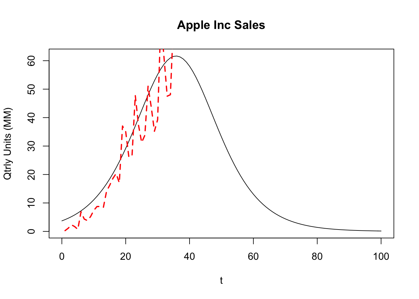
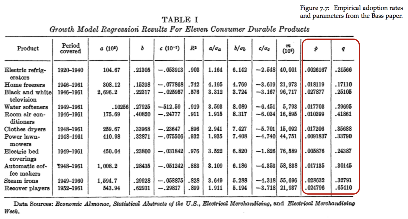
15.13 Comparison to other products
The estimated Apple coefficients are: \(p=0.0018\) and \(q=0.1148\). For several other products, the table below shows the estimated coefficients reported in Table I of the original Bass (1969) paper.
15.14 Sales Peak
It is easy to calculate the time at which adoptions will peak out. Differentiate \(f(t)\) with respect to \(t\), and set the result equal to zero, i.e.
\[ t^* = \mbox{argmax}_t f(t) \]
which is equivalent to the solution to \(f'(t)=0\).
The calculations are simple and give
\[ t^* = \frac{-1}{p+q}\; \ln(p/q) \]
Hence, for the values \(p=0.01\) and \(q=0.2\), we have
\[ t^* = \frac{-1}{0.01+0.2} \ln(0.01/0.2) = 14.2654 \; \mbox{years}. \]
If we examine the plot in the earlier Figure in the symbolic math section we see this to be where the graph peaks out.
For the Apple data, here is the computation of the sales peak, reported in number of quarters from inception.
#PEAK SALES TIME POINT (IN QUARTERS) FOR APPLE
tstar = -1/(p+q)*log(p/q)
print(tstar)## (Intercept)
## 35.7793915.15 Samsung Galaxy Phone Sales
#Read in Galaxy sales data
data = read.csv("DSTMAA_data/galaxy_sales.csv")
#Get coefficients
isales = data[,2]
cum_isales = cumsum(isales)
cum_isales2 = cum_isales^2
res = lm(isales ~ cum_isales+cum_isales2)
print(summary(res))
##
## Call:
## lm(formula = isales ~ cum_isales + cum_isales2)
##
## Residuals:
## Min 1Q Median 3Q Max
## -11.1239 -6.1774 0.4633 5.0862 13.2662
##
## Coefficients:
## Estimate Std. Error t value Pr(>|t|)
## (Intercept) 5.375e+01 4.506e+00 11.928 2.87e-10 ***
## cum_isales 7.660e-02 1.068e-02 7.173 8.15e-07 ***
## cum_isales2 -2.806e-05 5.074e-06 -5.530 2.47e-05 ***
## ---
## Signif. codes: 0 '***' 0.001 '**' 0.01 '*' 0.05 '.' 0.1 ' ' 1
##
## Residual standard error: 7.327 on 19 degrees of freedom
## Multiple R-squared: 0.8206, Adjusted R-squared: 0.8017
## F-statistic: 43.44 on 2 and 19 DF, p-value: 8.167e-08b = res$coefficients
#FIT THE MODEL
m1 = (-b[2]+sqrt(b[2]^2-4*b[1]*b[3]))/(2*b[3])
m2 = (-b[2]-sqrt(b[2]^2-4*b[1]*b[3]))/(2*b[3])
print(c(m1,m2))
## cum_isales cum_isales
## -578.9157 3308.9652m = max(m1,m2); print(m)## [1] 3308.965p = b[1]/m
q = -m*b[3]
print(c("p,q=",p,q))## (Intercept) cum_isales2
## "p,q=" "0.0162432614649845" "0.0928432001791269"#PLOT THE FITTED MODEL
nqtrs = 100
t=seq(0,nqtrs)
ff = D(FF,"t")
fn_f = eval(ff)*m
plot(t,fn_f,type="l",ylab="Qtrly Units (MM)",main="Samsung Galaxy Sales")
n = length(isales)
lines(1:n,isales,col="red",lwd=2,lty=2)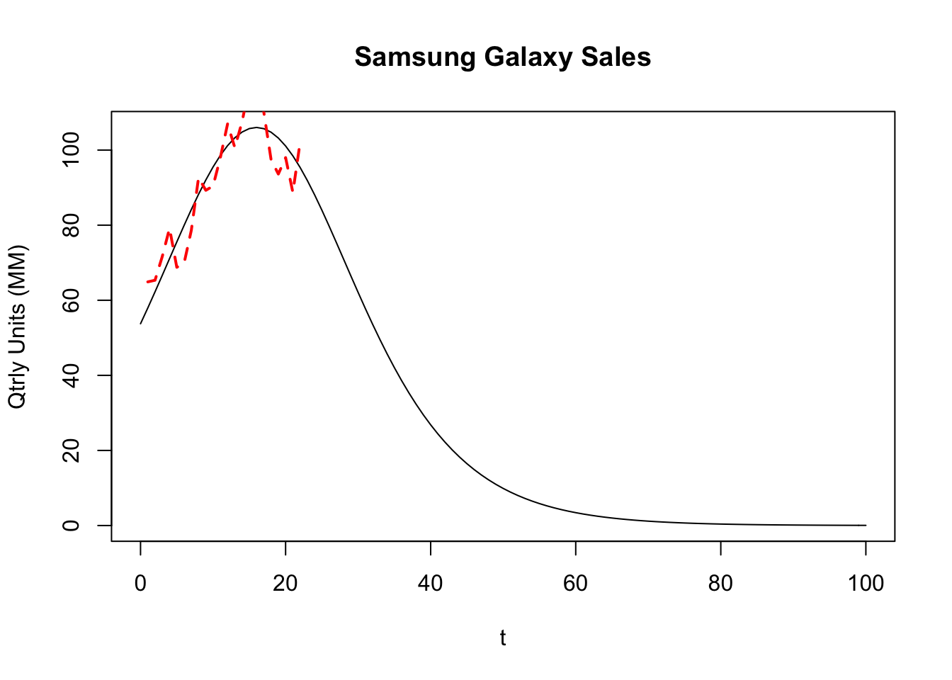
15.16 Global Semiconductor Sales
#Read in semiconductor sales data
data = read.csv("DSTMAA_data/semiconductor_sales.csv")

#Get coefficients
isales = data[,2]
cum_isales = cumsum(isales)
cum_isales2 = cum_isales^2
res = lm(isales ~ cum_isales+cum_isales2)
print(summary(res))
##
## Call:
## lm(formula = isales ~ cum_isales + cum_isales2)
##
## Residuals:
## Min 1Q Median 3Q Max
## -42.359 -12.415 0.698 12.963 45.489
##
## Coefficients:
## Estimate Std. Error t value Pr(>|t|)
## (Intercept) 5.086e+01 8.627e+00 5.896 3.76e-06 ***
## cum_isales 9.004e-02 9.601e-03 9.378 1.15e-09 ***
## cum_isales2 -6.878e-06 1.988e-06 -3.459 0.00196 **
## ---
## Signif. codes: 0 '***' 0.001 '**' 0.01 '*' 0.05 '.' 0.1 ' ' 1
##
## Residual standard error: 21.46 on 25 degrees of freedom
## Multiple R-squared: 0.9515, Adjusted R-squared: 0.9476
## F-statistic: 245.3 on 2 and 25 DF, p-value: < 2.2e-16b = res$coefficients
#FIT THE MODEL
m1 = (-b[2]+sqrt(b[2]^2-4*b[1]*b[3]))/(2*b[3])
m2 = (-b[2]-sqrt(b[2]^2-4*b[1]*b[3]))/(2*b[3])
print(c(m1,m2))## cum_isales cum_isales
## -542.4036 13633.3003m = max(m1,m2); print(m)## [1] 13633.3p = b[1]/m
q = -m*b[3]
print(c("p,q=",p,q))## (Intercept) cum_isales2
## "p,q=" "0.00373048366213552" "0.0937656034785294"#PLOT THE FITTED MODEL
nqtrs = 100
t=seq(0,nqtrs)
ff = D(FF,"t")
fn_f = eval(ff)*m
plot(t,fn_f,type="l",ylab="Annual Sales",main="Semiconductor Sales")
n = length(isales)
lines(1:n,isales,col="red",lwd=2,lty=2)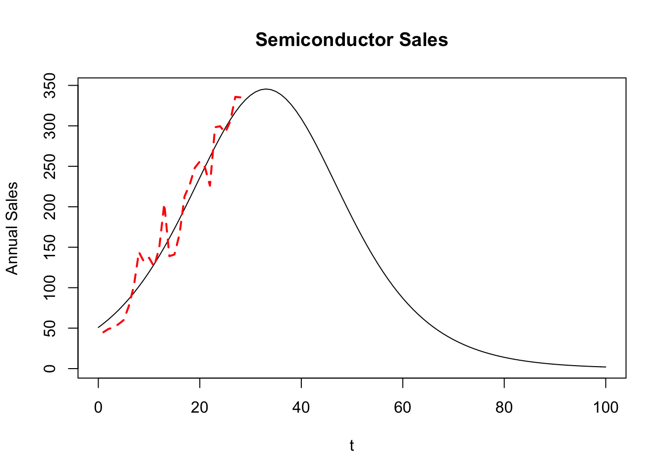
Show data frame:
df = as.data.frame(cbind(t,1988+t,fn_f))
print(df)
## t V2 fn_f
## 1 0 1988 50.858804
## 2 1 1989 55.630291
## 3 2 1990 60.802858
## 4 3 1991 66.400785
## 5 4 1992 72.447856
## 6 5 1993 78.966853
## 7 6 1994 85.978951
## 8 7 1995 93.503005
## 9 8 1996 101.554731
## 10 9 1997 110.145765
## 11 10 1998 119.282622
## 12 11 1999 128.965545
## 13 12 2000 139.187272
## 14 13 2001 149.931747
## 15 14 2002 161.172802
## 16 15 2003 172.872875
## 17 16 2004 184.981811
## 18 17 2005 197.435829
## 19 18 2006 210.156736
## 20 19 2007 223.051488
## 21 20 2008 236.012180
## 22 21 2009 248.916580
## 23 22 2010 261.629271
## 24 23 2011 274.003469
## 25 24 2012 285.883554
## 26 25 2013 297.108294
## 27 26 2014 307.514709
## 28 27 2015 316.942473
## 29 28 2016 325.238670
## 30 29 2017 332.262713
## 31 30 2018 337.891162
## 32 31 2019 342.022188
## 33 32 2020 344.579402
## 34 33 2021 345.514816
## 35 34 2022 344.810743
## 36 35 2023 342.480503
## 37 36 2024 338.567889
## 38 37 2025 333.145434
## 39 38 2026 326.311588
## 40 39 2027 318.186993
## 41 40 2028 308.910101
## 42 41 2029 298.632384
## 43 42 2030 287.513417
## 44 43 2031 275.716082
## 45 44 2032 263.402104
## 46 45 2033 250.728110
## 47 46 2034 237.842301
## 48 47 2035 224.881829
## 49 48 2036 211.970872
## 50 49 2037 199.219405
## 51 50 2038 186.722585
## 52 51 2039 174.560685
## 53 52 2040 162.799482
## 54 53 2041 151.490998
## 55 54 2042 140.674507
## 56 55 2043 130.377708
## 57 56 2044 120.618009
## 58 57 2045 111.403835
## 59 58 2046 102.735925
## 60 59 2047 94.608582
## 61 60 2048 87.010824
## 62 61 2049 79.927455
## 63 62 2050 73.340010
## 64 63 2051 67.227596
## 65 64 2052 61.567619
## 66 65 2053 56.336405
## 67 66 2054 51.509716
## 68 67 2055 47.063180
## 69 68 2056 42.972643
## 70 69 2057 39.214436
## 71 70 2058 35.765596
## 72 71 2059 32.604021
## 73 72 2060 29.708584
## 74 73 2061 27.059212
## 75 74 2062 24.636929
## 76 75 2063 22.423878
## 77 76 2064 20.403319
## 78 77 2065 18.559614
## 79 78 2066 16.878199
## 80 79 2067 15.345546
## 81 80 2068 13.949122
## 82 81 2069 12.677336
## 83 82 2070 11.519492
## 84 83 2071 10.465737
## 85 84 2072 9.507005
## 86 85 2073 8.634969
## 87 86 2074 7.841989
## 88 87 2075 7.121062
## 89 88 2076 6.465778
## 90 89 2077 5.870270
## 91 90 2078 5.329179
## 92 91 2079 4.837608
## 93 92 2080 4.391088
## 94 93 2081 3.985542
## 95 94 2082 3.617252
## 96 95 2083 3.282831
## 97 96 2084 2.979193
## 98 97 2085 2.703528
## 99 98 2086 2.453280
## 100 99 2087 2.226120
## 101 100 2088 2.01993215.17 Extensions
The Bass model has been extended to what is known as the generalized Bass model in a paper by Bass, Krishnan, and Jain (1994). The idea is to extend the model to the following equation:
\[ \frac{f(t)}{1-F(t)} = [p+q\; F(t)] \; x(t) \]
where \(x(t)\) stands for current marketing effort. This additional variable allows (i) consideration of effort in the model, and (ii) given the function \(x(t)\), it may be optimized.
The Bass model comes from a deterministic differential equation. Extensions to stochastic differential equations need to be considered.
See also the paper on Bayesian inference in Bass models by Boatwright and Kamakura (2003).
- Bass, Frank. (1969). “A New Product Growth Model for Consumer Durables,” Management Science 16, 215–227.
- Bass, Frank., Trichy Krishnan, and Dipak Jain (1994). “Why the Bass Model Without Decision Variables,” Marketing Science 13, 204–223.
- Boatwright, Lee., and Wagner Kamakura (2003). “Bayesian Model for Prelaunch Sales Forecasting of Recorded Music,” Management Science 49(2), 179–196.
15.18 Trading off \(p\) vs \(q\)
In the Bass model, if the coefficient of imitation increases relative to the coefficient of innovation, then which of the following is the most valid?
- the peak of the product life cycle occurs later.
- the peak of the product life cycle occurs sooner.
- there may be an increasing chance of two life-cycle peaks.
- the peak may occur sooner or later, depending on the coefficient of innovation.
Using peak time formula, substitute \(x=q/p\):
\[ t^*=\frac{-1}{p+q} \ln(p/q) = \frac{\ln(q/p)}{p+q} = \frac{1}{p} \; \frac{\ln(q/p)}{1+q/p} = \frac{1}{p}\; \frac{\ln(x)}{1+x} \]
Differentiate with regard to x (we are interested in the sign of the first derivative \(\partial t^*/\partial q\), which is the same as sign of \(\partial t^*/\partial x\)):
\[ \frac{\partial t^*}{\partial x} = \frac{1}{p}\left[\frac{1}{x(1+x)}-\frac{\ln x}{(1+x)^2}\right]=\frac{1+x-x\ln x}{px(1+x)^2} \]
From the Bass model we know that \(q > p > 0\), i.e. \(x>1\), otherwise we could get negative values of acceptance or shape without maximum in the \(0 \le F < 1\) area. Therefore, the sign of \(\partial t^*/\partial x\) is same as:
\[ sign\left(\frac{\partial t^*}{\partial x}\right) = sign(1+x-x\ln x), ~~~ x>1 \]
But this non-linear equation
\[ 1+x-x\ln x=0, ~~~ x>1 \]
has a root \(x \approx 3.59\).
In other words, the derivative \(\partial t^* / \partial x\) is negative when \(x > 3.59\) and positive when \(x < 3.59\). For low values of \(x=q/p\), an increase in the coefficient of imitation \(q\) increases the time to sales peak, and for high values of \(q/p\) the time decreases with increasing \(q\). So the right answer for the question appears to be “it depends on values of \(p\) and \(q\)”.
t = seq(0,5,0.1)
p = 0.1; q=0.22
plot(t,f(p,q,t),type="l",col="blue",lwd=2)
p = 0.1; q=0.20
lines(t,f(p,q,t),type="l",col="red",lwd=2)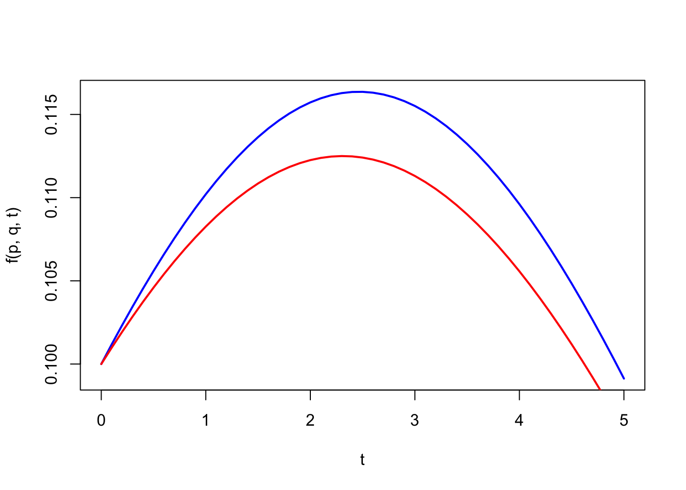
In the Figure, when \(x\) gets smaller, the peak is earlier.