24. Text Classification with GLMNet#
Classification using regularized elastic net.
from google.colab import drive
drive.mount('/content/drive')  # Add My Drive/<>

import os
os.chdir('drive/My Drive')
os.chdir('Books_Writings/NLPBook/')
Mounted at /content/drive
%%capture
%pylab inline
import pandas as pd
import os
%load_ext rpy2.ipython
# !pip install -q condacolab
# import condacolab
# condacolab.install()
24.1. Text Classification using GLMNet#
The large movie review dataset is here: https://ai.stanford.edu/~amaas/data/sentiment/
For an excellent description of glmnet see: https://web.stanford.edu/~hastie/glmnet/glmnet_alpha.html
Let’s move over to the R program to run GLMNet, as it was written for that environmemt. We will execute the %%R code blocks in a separate notebook with a R kernel.
%%R
install.packages(c("data.table","magrittr"), quiet=TRUE)
# !conda install -c r r-data.table r-magrittr -y
%%R
install.packages("glmnet", quiet=TRUE) # long install
# !conda install -c conda-forge glmnet -y
also installing the dependencies ‘iterators’, ‘foreach’, ‘shape’, ‘RcppEigen’
%%R
install.packages(c("text2vec"), quiet=TRUE) # VERY LONG INSTALL
# !conda install -c conda-forge r-text2vec -y   # Need the -y to not have to answer 'y' after packages are detected
also installing the dependencies ‘MatrixExtra’, ‘float’, ‘RhpcBLASctl’, ‘RcppArmadillo’, ‘rsparse’, ‘mlapi’, ‘lgr’
%%R
library(text2vec)
library(data.table)
data.table 1.17.8 using 1 threads (see ?getDTthreads). Latest news: r-datatable.com
%%R
data("movie_review")
setDT(movie_review)
setkey(movie_review, id)
set.seed(2016L)
all_ids = movie_review$id
train_ids = sample(all_ids, 4000)
test_ids = setdiff(all_ids, train_ids)
train = movie_review[J(train_ids)]
test = movie_review[J(test_ids)]

print(head(train))
id sentiment
<char> <int>
1: 6748_8 1
2: 1294_7 1
3: 11206_10 1
4: 1217_10 1
5: 10395_8 1
6: 6531_8 1
review
<char>
1: New York police detective Mark Dixon (Dana Andrews) is a guy who has to deal with his own demons on a daily basis at the same time as coping with the normal ups and downs of everyday life. The strain produced by his internal struggle and his intense hatred of criminals, leads him to make serious errors of judgement and to fail to recognise the need for any code of conduct to be adhered to in his dealings with people on the wrong side of the law. He has a track record of treating suspects and known criminals with gross brutality and this has brought him into conflict with his superior officers who have censured him for the amount of violence he has regularly used. Dixon cannot reconcile these calls for restraint with his own extreme and irrational hatred of all criminals. He is tormented by the fact that his father was a criminal and has been left with a powerful need to live down his father's reputation and to avoid fulfilling the low expectations that many people have of him as a consequence.<br /><br />When a rich Texan is murdered following an evening's gambling run by gangster Tommy Scalise (Gary Merrill), Dixon is assigned to the case. Scalise tells Dixon's superior officer Detective Lieutenant Thomas (Karl Malden) that the victim had been accompanied by Ken Paine (Craig Stevens) and his wife Morgan (Gene Tierney) and that Paine had committed the murder. Dixon goes to Paine's apartment and questions the suspect who is both inebriated and uncooperative and when Paine punches him, Dixon retaliates and Paine collapses and dies. Dixon goes on to dispose of the body in a nearby river. Paine's wife is questioned and after describing what had happened at Scalise's place, adds that her father had gone to Paine's apartment later that night to take issue with him about the fact that she'd returned home with facial bruising. Paine had previously attacked her on a number of occasions and her father, Jiggs Taylor (Tom Tully), had threatened that if it happened again he would beat Paine up. This information leads to Taylor being arrested and charged with murder. Nobody accepts Dixon's explanation that Scalise had killed the Texan and then had Paine killed to eliminate him as a witness.<br /><br />Dixon continues to make various attempts to get Scalise convicted but eventually realises that the only way to successfully achieve his goal is to write a confession about his own role in Paine's death and the cover up. He does this and also records that he is going alone to confront Scalise so that the police can arrest the gangster for Dixon's murder. The confrontation with Scalise and the eventual means by which Dixon achieves his own redemption, provide a tense and fitting conclusion to this gritty thriller.<br /><br />Dana Andrews' strained and preoccupied expressions convey his character's perpetually troubled nature and his anxieties as he deals with a series of misfortunes which include and follow Paine's accidental death. Dixon, however, isn't the only one to experience misfortune as Morgan, a successful model loses her job because of all the trouble surrounding her. Her father, who'd some years earlier been awarded a diploma for assisting the police, unjustly finds himself charged with a crime he did not commit. Ken Paine who'd been a war hero had experienced unemployment and a loss of self esteem which led to alcoholism and wife beating and Scalise who'd been set up in business by Dixon's father also suffers his own misfortunes.<br /><br />\\"Where The Sidewalk Ends\\" is a thoroughly engaging tale involving a group of interesting and diverse characters and a main protagonist who is the absolute personification of moral ambiguity.
2: Unremittingly bleak and depressing, the film evokes as well as could be desired the legendary misery and emptiness that characterised Houellebecq's controversial novel of the same name. Like many French films, its manner is one of wistful profundity but it is painfully slow - or should that be, slowly painful? While this is an excellent and challenging film, it is not an enjoyable one and its difficult to think of any time when one might be in the 'right' mood to see it.
3: I have not seen this movie! At least not in its entirety. I have seen a few haunting clips which have left me gagging to see it all. One sequence remains in my memory to this day. A (very convincing looking) spacecraft is orbiting the dark side of the moon. The pilot releases a flash device in order to photograph the hidden surface below him. The moon flashes into visability . . . . and for a few seconds there it is. Parallel lines, squares, Could it be .. then the light fades and the brief glimse of ...what... has gone and it is time for the spacecraft to return to Earth. Wonderful. I have seen some other clips too but would LOVE to obtain the full movie.
4: I was worried that my daughter might get the wrong idea. I think the \\"Dark-Heart\\" character is a little on the rough side and I don't like the way he shape-shifts into a \\"mean\\" frog, fox, boy I was wrong, This movie was made for my kid, not for me. She \\"gets it\\" when it went over (under?) my head. Of course I don't \\"get it\\". This isn't one of the NEW kids movies that adults will ALSO enjoy. This is straight for the young ones, and the crew knew what they were doing. There isn't any political junk ether. There's no magic key that will save the world from ourselves, nobody has the right to access excess, and everyone isn't happy all the time. And as a side benefit, nobody DIES! russwill.
5: A fantastic Arabian adventure. A former king, Ahmad, and his best friend, the thief Abu (played by Sabu of Black Narcissus) search for Ahmad's love interest, who has been stolen by the new king, Jaffar (Conrad Veidt). There's hardly a down moment here. It's always inventing new adventures for the heroes. Personally, I found Ahmad and his princess a little boring (there's no need to ask why John Justin, who plays Ahmad, is listed fourth in the credits). Conrad Veidt, always a fun actor, makes a great villain, and Sabu is a lot of fun as the prince of thieves, who at one point finds a genie in a bottle. I also really loved Miles Malleson as the Sultan of Basra, the father of the princess. He collects amazing toys from around the world. Jaffar bribes him for his daughter's hand with a mechanical flying horse. This probably would count as one of the great children's films of all time, but the special effects are horribly dated nowadays. Kids will certainly deride the superimposed images when Abu and the genie are on screen together. And the scene with the giant spider looks especially awful. Although most of the younger generation probably thinks that King Kong looks bad at this point in time, Willis O'Brien's stop-motion animation is a thousand times better than a puppet on a string that doesn't even look remotely like a spider. 8/10.
6: I really liked this movie...it was cute. I enjoyed it, but if you didn't, that is your fault. Emma Roberts played a good Nancy Drew, even though she isn't quite like the books. The old fashion outfits are weird when you see them in modern times, but she looks good on them. To me, the rich girls didn't have outfits that made them look rich. I mean, it looks like they got all the clothes -blindfolded- at a garage sale and just decided to put it on all together. All of the outfits were tacky, especially when they wore the penny loafers with their regular outfits. I do not want to make the movie look bad, because it definitely wasn't! Just go to the theater and watch it!!! You will enjoy it!
%%R
# Get from R into python, through csv file
write.csv(movie_review, "NLP_data/movie_review.csv", row.names=FALSE)
mr = pd.read_csv("NLP_data/movie_review.csv")
print(mr.shape)
mr.head()
(5000, 3)
| id | sentiment | review | |
|---|---|---|---|
| 0 | 10000_8 | 1 | Homelessness (or Houselessness as George Carli... |
| 1 | 10001_4 | 0 | This film lacked something I couldn't put my f... |
| 2 | 10004_3 | 0 | \"It appears that many critics find the idea o... |
| 3 | 10004_8 | 1 | This isn't the comedic Robin Williams, nor is ... |
| 4 | 10006_4 | 0 | I don't know who to blame, the timid writers o... |
%%R
prep_fun = tolower
tok_fun = word_tokenizer

#Create an iterator to pass to the create_vocabulary function
it_train = itoken(train$review,
             preprocessor = prep_fun,
             tokenizer = tok_fun,
             ids = train$id,
             progressbar = FALSE)

#Now create a vocabulary
vocab = create_vocabulary(it_train)
print(vocab)
Number of docs: 4000
0 stopwords:  ...
ngram_min = 1; ngram_max = 1
Vocabulary:
         term term_count doc_count
       <char>      <int>     <int>
    1:   0.02          1         1
    2:    0.3          1         1
    3:   0.48          1         1
    4:    0.5          1         1
    5:   0.89          1         1
   ---
38457:     to      22238      3792
38458:     of      23604      3787
38459:      a      26609      3876
38460:    and      26950      3863
38461:    the      54281      3971
%%R
vectorizer = vocab_vectorizer(vocab)
dtm_train = create_dtm(it_train, vectorizer)
print(dim(as.matrix(dtm_train)))
vocab = create_vocabulary(it_train, ngram = c(1, 2))
print(vocab)
[1]  4000 38461
Number of docs: 4000
0 stopwords:  ...
ngram_min = 1; ngram_max = 2
Vocabulary:
            term term_count doc_count
          <char>      <int>     <int>
     1:     0.02          1         1
     2: 0.02_out          1         1
     3:   0.0_10          1         1
     4: 0.0_it's          1         1
     5:      0.3          1         1
    ---
406974:       to      22238      3792
406975:       of      23604      3787
406976:        a      26609      3876
406977:      and      26950      3863
406978:      the      54281      3971
In addition: Warning message:
In asMethod(object) :
  sparse->dense coercion: allocating vector of size 1.1 GiB
%%R
library(glmnet)
library(magrittr)
NFOLDS = 5

vocab2 = vocab %>% prune_vocabulary(term_count_min = 10,
                   doc_proportion_max = 0.5)
print(vocab2)
Number of docs: 4000
0 stopwords:  ...
ngram_min = 1; ngram_max = 2
Vocabulary:
         term term_count doc_count
       <char>      <int>     <int>
    1:   1948         10         9
    2:   1951         10         9
    3:   1966         10         6
    4: 1970_s         10         9
    5:   1977         10        10
   ---
17700:   like       3374      1920
17701:   they       3403      1642
17702:     by       3642      1885
17703:     he       4240      1571
17704:    his       4688      1721
Loading required package: Matrix
Loaded glmnet 4.1-10
%%R
bigram_vectorizer = vocab_vectorizer(vocab2)
dtm_train = create_dtm(it_train, bigram_vectorizer)
res = cv.glmnet(x = dtm_train, y = train[['sentiment']],
                 family = 'binomial',
                 alpha = 1,
                 type.measure = "auc",
                 nfolds = NFOLDS,
                 thresh = 1e-3,
                 maxit = 1e3)
plot(res)
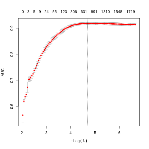
%%R
print(names(res))
cat("AUC (area under curve):")
print(max(res$cvm))
 [1] "lambda"     "cvm"        "cvsd"       "cvup"       "cvlo"
 [6] "nzero"      "call"       "name"       "glmnet.fit" "lambda.min"
[11] "lambda.1se" "index"
AUC (area under curve):[1] 0.9179888
%%R
#Out-of-sample test
it_test = test$review %>%
  prep_fun %>%
  tok_fun %>%
  itoken(ids = test$id,
         # turn off progressbar because it won't look nice in rmd
         progressbar = FALSE)

dtm_test = create_dtm(it_test, bigram_vectorizer)
preds = predict(res, dtm_test, type = 'response')[,1]
glmnet:::auc(test$sentiment, preds)
[1] 0.9164907
%%R
accuracy = mean(test$sentiment==round(preds))
accuracy
[1] 0.831
%%R
res = glmnet(x = dtm_train,
             y = train[['sentiment']],
             family = 'binomial',
             alpha = 1,
             thresh = 1e-3,
             maxit = 1e3)

print(names(res))
print(res)
 [1] "a0"         "beta"       "df"         "dim"        "lambda"
 [6] "dev.ratio"  "nulldev"    "npasses"    "jerr"       "offset"
[11] "classnames" "call"       "nobs"

Call:  glmnet(x = dtm_train, y = train[["sentiment"]], family = "binomial",      alpha = 1, thresh = 0.001, maxit = 1000)

      Df  %Dev   Lambda
1      0  0.00 0.130300
2      1  0.44 0.124400
3      1  0.83 0.118700
4      2  1.25 0.113300
5      2  1.78 0.108200
6      3  2.32 0.103300
7      3  3.05 0.098570
8      3  3.71 0.094090
9      3  4.33 0.089820
10     4  5.04 0.085740
11     5  5.79 0.081840
12     6  6.63 0.078120
13     6  7.42 0.074570
14     7  8.26 0.071180
15     7  9.05 0.067940
16     9  9.95 0.064860
17    11 10.85 0.061910
18    12 11.76 0.059090
19    14 12.75 0.056410
20    17 13.74 0.053840
21    22 14.81 0.051400
22    24 15.94 0.049060
23    26 17.03 0.046830
24    26 18.11 0.044700
25    35 19.23 0.042670
26    37 20.35 0.040730
27    43 21.51 0.038880
28    49 22.70 0.037110
29    55 23.89 0.035430
30    62 25.10 0.033820
31    68 26.32 0.032280
32    74 27.56 0.030810
33    78 28.77 0.029410
34    87 29.96 0.028070
35   101 31.18 0.026800
36   112 32.40 0.025580
37   123 33.63 0.024420
38   139 34.90 0.023310
39   158 36.19 0.022250
40   176 37.50 0.021240
41   193 38.83 0.020270
42   213 40.18 0.019350
43   230 41.54 0.018470
44   265 42.92 0.017630
45   286 44.32 0.016830
46   306 45.74 0.016070
47   335 47.16 0.015340
48   371 48.61 0.014640
49   411 50.07 0.013970
50   457 51.56 0.013340
51   485 53.06 0.012730
52   513 54.54 0.012150
53   554 56.01 0.011600
54   583 57.46 0.011070
55   631 58.88 0.010570
56   672 60.30 0.010090
57   715 61.70 0.009631
58   768 63.08 0.009193
59   814 64.44 0.008775
60   851 65.78 0.008376
61   886 67.10 0.007996
62   922 68.39 0.007632
63   962 69.65 0.007285
64   991 70.87 0.006954
65  1041 72.07 0.006638
66  1069 73.23 0.006336
67  1095 74.35 0.006048
68  1129 75.44 0.005774
69  1167 76.49 0.005511
70  1193 77.49 0.005261
71  1223 78.46 0.005022
72  1252 79.40 0.004793
73  1281 80.30 0.004575
74  1310 81.16 0.004367
75  1339 82.00 0.004169
76  1355 82.79 0.003979
77  1378 83.56 0.003799
78  1391 84.29 0.003626
79  1413 84.99 0.003461
80  1443 85.67 0.003304
81  1463 86.31 0.003154
82  1483 86.93 0.003010
83  1506 87.52 0.002874
84  1529 88.09 0.002743
85  1548 88.63 0.002618
86  1570 89.15 0.002499
87  1595 89.64 0.002386
88  1613 90.12 0.002277
89  1631 90.57 0.002174
90  1648 91.00 0.002075
91  1669 91.42 0.001981
92  1680 91.81 0.001891
93  1691 92.19 0.001805
94  1703 92.55 0.001723
95  1714 92.89 0.001644
96  1719 93.21 0.001570
97  1726 93.52 0.001498
98  1741 93.82 0.001430
99  1754 94.10 0.001365
100 1762 94.37 0.001303
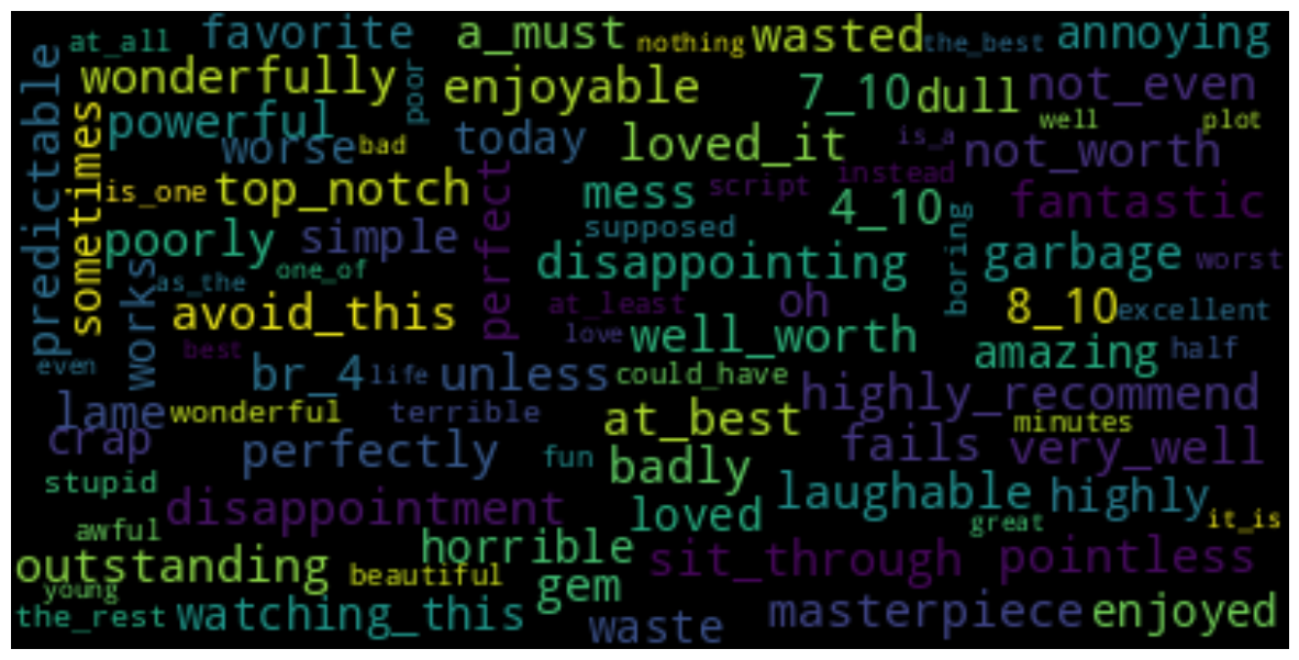
%%R
f = res$beta[,35]   # feature coefficients
non0f = f[which(f!=0)]
words = names(non0f)
words
  [1] "7_10"             "br_4"             "4_10"
  [4] "well_worth"       "top_notch"        "8_10"
  [7] "loved_it"         "not_worth"        "wonderfully"
 [10] "avoid_this"       "at_best"          "sit_through"
 [13] "outstanding"      "highly_recommend" "disappointment"
 [16] "gem"              "a_must"           "disappointing"
 [19] "laughable"        "garbage"          "wasted"
 [22] "masterpiece"      "fails"            "pointless"
 [25] "mess"             "poorly"           "lame"
 [28] "badly"            "7"                "not_even"
 [31] "unless"           "powerful"         "perfectly"
 [34] "predictable"      "enjoyable"        "very_well"
 [37] "8"                "fantastic"        "watching_this"
 [40] "dull"             "today"            "annoying"
 [43] "crap"             "simple"           "horrible"
 [46] "amazing"          "favorite"         "highly"
 [49] "enjoyed"          "oh"               "sometimes"
 [52] "works"            "waste"            "loved"
 [55] "perfect"          "worse"            "supposed"
 [58] "boring"           "terrible"         "wonderful"
 [61] "the_rest"         "stupid"           "could_have"
 [64] "awful"            "half"             "at_all"
 [67] "poor"             "beautiful"        "instead"
 [70] "is_one"           "excellent"        "each"
 [73] "at_least"         "worst"            "fun"
 [76] "minutes"          "script"           "both"
 [79] "the_best"         "young"            "nothing"
 [82] "as_the"           "life"             "love"
 [85] "best"             "plot"             "any"
 [88] "could"            "one_of"           "don't"
 [91] "him"              "bad"              "great"
 [94] "also"             "it_is"            "well"
 [97] "would"            "even"             "no"
[100] "is_a"             "very"
%%R
wordcount = abs(non0f)
wordcount
            7_10             br_4             4_10       well_worth
    0.1737067602     0.1537751279     0.3880592592     0.3721005173
       top_notch             8_10         loved_it        not_worth
    0.1157643996     0.1437147779     0.1253946762     0.2077053287
     wonderfully       avoid_this          at_best      sit_through
    0.0079554286     0.0036507740     0.0214432297     0.0607129705
     outstanding highly_recommend   disappointment              gem
    0.0047577937     0.0988630171     0.0818577027     0.1342509079
          a_must    disappointing        laughable          garbage
    0.1715726294     0.1759929460     0.2081529486     0.1119382095
          wasted      masterpiece            fails        pointless
    0.3001975722     0.0041195927     0.0058318612     0.1993796544
            mess           poorly             lame            badly
    0.2689532518     0.2970575815     0.1526924581     0.3828920110
               7         not_even           unless         powerful
    0.0088373086     0.0361185501     0.2174626015     0.0182370459
       perfectly      predictable        enjoyable        very_well
    0.2586627701     0.2015641465     0.0005408451     0.0061813890
               8        fantastic    watching_this             dull
    0.0231843822     0.0202758208     0.1296938462     0.4398502264
           today         annoying             crap           simple
    0.0101171266     0.2076269110     0.1254315229     0.1017981031
        horrible          amazing         favorite           highly
    0.1749285322     0.0893412037     0.1761840213     0.2677309677
         enjoyed               oh        sometimes            works
    0.0866742986     0.0573299889     0.0130417042     0.0027208961
           waste            loved          perfect            worse
    0.8885586757     0.0632260958     0.3187142797     0.4235111175
        supposed           boring         terrible        wonderful
    0.1548044674     0.1784309088     0.2657562368     0.2533313571
        the_rest           stupid       could_have            awful
    0.0094969163     0.2870561447     0.0752214545     0.5492803513
            half           at_all             poor        beautiful
    0.0443046289     0.0788475277     0.5598074988     0.1687722767
         instead           is_one        excellent             each
    0.0645239351     0.0062682732     0.4474954046     0.0144275366
        at_least            worst              fun          minutes
    0.0528647144     0.8213753494     0.0923106106     0.0443434725
          script             both         the_best            young
    0.0985778858     0.0950806452     0.1126035090     0.0138495029
         nothing           as_the             life             love
    0.2215979214     0.0234677051     0.1088309271     0.0524184779
            best             plot              any            could
    0.1377961401     0.0291256214     0.1053974100     0.0401790144
          one_of            don't              him              bad
    0.1274950684     0.0128343287     0.0048012888     0.4182907097
           great             also            it_is             well
    0.3300346392     0.0116133245     0.0023719491     0.0332481484
           would             even               no             is_a
    0.0176289221     0.0032845981     0.0689067060     0.1087572724
            very
    0.0642045124
%%R
print(names(vocab2))
all_words = vocab2$term
all_term_count = vocab2$term_count
all_doc_count = vocab2$doc_count
[1] "term" "term_count" "doc_count"
words = %Rget words
wordcount = %Rget wordcount
all_words = %Rget all_words
all_term_count = %Rget all_term_count
all_doc_count = %Rget all_doc_count
all_words = array([j for j in all_words])
all_term_count = array([j for j in all_term_count])
all_doc_count = array([j for j in all_doc_count])
text = ""
for w in words:
    n = all_term_count[all_words==w][0]
    n = 1
    if n>0:
        for j in range(n):
            text = text + " " + w
from wordcloud import WordCloud
wordcloud = WordCloud(max_font_size=15).generate(text)

#Use pyplot from matplotlib
figure(figsize=(15,8))
pyplot.imshow(wordcloud, interpolation='bilinear')
pyplot.axis("off")
(np.float64(-0.5), np.float64(399.5), np.float64(199.5), np.float64(-0.5))