
8. Machine Learning: A Quick Introduction#
A quick recap of machine learning before we get started with NLP.
8.1. Jupyter Extensions#
These allow using the notebooks in myriad ways, see: https://blog.jupyter.org/99-ways-to-extend-the-jupyter-ecosystem-11e5dab7c54
from google.colab import drive
drive.mount('/content/drive')  # Add My Drive/<>

import os
os.chdir('drive/My Drive')
os.chdir('Books_Writings/NLPBook/')
Mounted at /content/drive
%%capture
# %pylab inline
import pandas as pd
import os
import numpy as np
import matplotlib.pyplot as plt
from IPython.display import Image
Image("NLP_images/ML_AI.png", width=700)
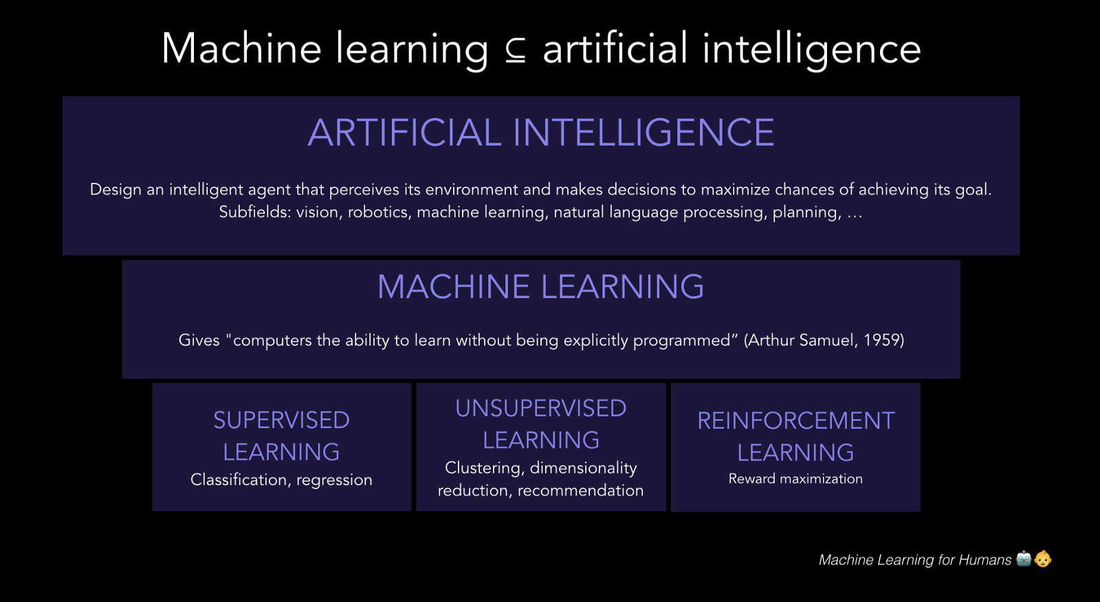
https://medium.com/machine-learning-for-humans/why-machine-learning-matters-6164faf1df12
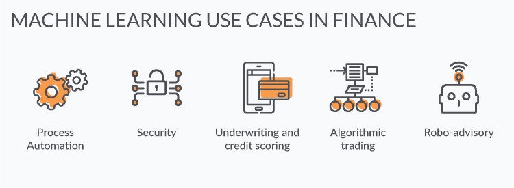
8.2. 5 Applications of ML in Finance#
https://www.verypossible.com/blog/5-applications-of-machine-learning-in-finance
https://towardsdatascience.com/machine-learning-in-finance-why-what-how-d524a2357b56
Image("NLP_images/ML_use_cases.jpg", width=600)
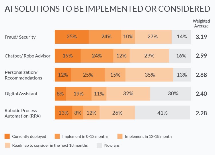
Image("NLP_images/AI_solutions.jpg", width=600)
8.3. Many Applications of ML in Finance#
Fraud prevention
Risk management
Investment predictions
Customer service
Digital assistants
Marketing
Network security
Loan underwriting
Algorithmic trading
Process automation
Document interpretation
Content creation
Trade settlements
Money-laundering prevention
Custom machine learning solutions
https://igniteoutsourcing.com/fintech/machine-learning-in-finance/
For projects, start looking at Kaggle for finance datasets you may be able to use.
8.4. J.P. Morgan Guide to ML in Finance#
https://news.efinancialcareers.com/uk-en/285249/machine-learning-and-big-data-j-p-morgan
“You won’t need to be a machine learning expert, you will need to be an excellent quant and an excellent programmer
J.P. Morgan says the skillset for the role of data scientists is virtually the same as for any other quantitative researchers. Existing buy side and sell side quants with backgrounds in computer science, statistics, maths, financial engineering, econometrics and natural sciences should therefore be able to reinvent themselves. Expertise in quantitative trading strategies will be the crucial skill. “It is much easier for a quant researcher to change the format/size of a dataset, and employ better statistical and Machine Learning tools, than for an IT expert, silicon valley entrepreneur, or academic to learn how to design a viable trading strategy,” say Kolanovic and Krishnamacharc.”
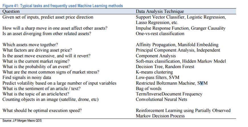
8.5. ML Tasks in Finance#
Image("NLP_images/JPMorgan-machine-learning-2.jpg", width=600)
8.6. ML with NLP#
Credit scoring, sentiment analysis, document search: https://emerj.com/ai-sector-overviews/natural-language-processing-applications-in-finance-3-current-applications/
Gather real-time intelligence on specific stocks; Provide key hire alerts; Monitor company sentiment; Anticipate client concerns; Upgrade quality of analyst reporting; Understand and respond to news events; Detect insider trading: https://www.ibm.com/blogs/watson/2016/06/natural-language-processing-transforming-financial-industry-2/
Ravenpack: https://www.ravenpack.com/; https://www.ravenpack.com/research/browse/
8.7. scikit-learn: Python’s one-stop shop for ML#
8.8. Supervised Learning Models#
Linear Models
Logistic Regression
Discriminant Analysis
Bayes Classifier
Support Vector Machines
Nearest Neighbors (kNN)
Decision Trees
Neural Networks
8.9. Unsupervised Learning Models#
8.9.1. Clustering#
K-means
Hierarchical clustering
8.9.2. Dimension Reduction#
Principal Components Analysis
Factor Analysis
Autoencoders
8.10. Ensemble Methods#
Bagging
Stacking
Boosting
8.11. Small Business Association (SBA) Loans Dataset#
#Import the SBA Loans dataset
pd.set_option('display.max_columns', 500)
sba = pd.read_csv("NLP_data/SBA.csv")
print(sba.columns)
print(sba.shape)
sba.head()
Index(['LoanID', 'GrossApproval', 'SBAGuaranteedApproval', 'subpgmdesc',
       'ApprovalFiscalYear', 'InitialInterestRate', 'TermInMonths',
       'ProjectState', 'BusinessType', 'LoanStatus', 'RevolverStatus',
       'JobsSupported'],
      dtype='object')
(527700, 12)
| LoanID | GrossApproval | SBAGuaranteedApproval | subpgmdesc | ApprovalFiscalYear | InitialInterestRate | TermInMonths | ProjectState | BusinessType | LoanStatus | RevolverStatus | JobsSupported | |
|---|---|---|---|---|---|---|---|---|---|---|---|---|
| 0 | 733784 | 50000 | 25000 | FA$TRK (Small Loan Express) | 2006 | 11.25 | 84 | IN | CORPORATION | CANCLD | 1 | 4 |
| 1 | 733785 | 35000 | 17500 | FA$TRK (Small Loan Express) | 2006 | 12.00 | 84 | IL | CORPORATION | CANCLD | 0 | 3 |
| 2 | 733786 | 15000 | 7500 | FA$TRK (Small Loan Express) | 2006 | 12.00 | 84 | WV | INDIVIDUAL | CANCLD | 0 | 4 |
| 3 | 733787 | 16000 | 13600 | Community Express | 2006 | 11.50 | 84 | MD | CORPORATION | PIF | 0 | 1 |
| 4 | 733788 | 16000 | 13600 | Community Express | 2006 | 11.50 | 84 | MD | CORPORATION | CANCLD | 0 | 1 |
8.12. Feature Engineering#
#Feature engineering
sba["GuaranteePct"] = sba.SBAGuaranteedApproval.astype("float")/sba.GrossApproval.astype("float")
X = sba[['ApprovalFiscalYear', 'InitialInterestRate', 'TermInMonths',
        'RevolverStatus','JobsSupported','GuaranteePct']]

x1 = pd.get_dummies(sba.subpgmdesc, dtype=int)
X = pd.concat([X,x1],axis=1)

x2 = pd.get_dummies(sba.BusinessType, dtype=int)
X = pd.concat([X,x2],axis=1)

X.head()
| ApprovalFiscalYear | InitialInterestRate | TermInMonths | RevolverStatus | JobsSupported | GuaranteePct | 509 - DEALER FLOOR PLAN | Community Advantage Initiative | Community Express | Contract Guaranty | EXPORT IMPORT HARMONIZATION | FA$TRK (Small Loan Express) | Guaranty | Gulf Opportunity | International Trade - Sec, 7(a) (16) | Lender Advantage Initiative | Patriot Express | Revolving Line of Credit Exports - Sec. 7(a) (14) | Rural Lender Advantage | Seasonal Line of Credit | Small Asset Based | Small General Contractors - Sec. 7(a) (9) | Standard Asset Based | CORPORATION | INDIVIDUAL | PARTNERSHIP | |
|---|---|---|---|---|---|---|---|---|---|---|---|---|---|---|---|---|---|---|---|---|---|---|---|---|---|---|
| 0 | 2006 | 11.25 | 84 | 1 | 4 | 0.50 | 0 | 0 | 0 | 0 | 0 | 1 | 0 | 0 | 0 | 0 | 0 | 0 | 0 | 0 | 0 | 0 | 0 | 1 | 0 | 0 |
| 1 | 2006 | 12.00 | 84 | 0 | 3 | 0.50 | 0 | 0 | 0 | 0 | 0 | 1 | 0 | 0 | 0 | 0 | 0 | 0 | 0 | 0 | 0 | 0 | 0 | 1 | 0 | 0 |
| 2 | 2006 | 12.00 | 84 | 0 | 4 | 0.50 | 0 | 0 | 0 | 0 | 0 | 1 | 0 | 0 | 0 | 0 | 0 | 0 | 0 | 0 | 0 | 0 | 0 | 0 | 1 | 0 |
| 3 | 2006 | 11.50 | 84 | 0 | 1 | 0.85 | 0 | 0 | 1 | 0 | 0 | 0 | 0 | 0 | 0 | 0 | 0 | 0 | 0 | 0 | 0 | 0 | 0 | 1 | 0 | 0 |
| 4 | 2006 | 11.50 | 84 | 0 | 1 | 0.85 | 0 | 0 | 1 | 0 | 0 | 0 | 0 | 0 | 0 | 0 | 0 | 0 | 0 | 0 | 0 | 0 | 0 | 1 | 0 | 0 |
8.13. Logistic Regression (Logit)#
8.13.1. Limited Dependent Variables#
The dependent variable may be discrete, and could be binomial or multinomial. That is, the dependent variable is limited. In such cases, we need a different approach.
Discrete dependent variables are a special case of limited dependent variables. The Logit model we look at here is a discrete dependent variable model. Such models are also often called qualitative response (QR) models.
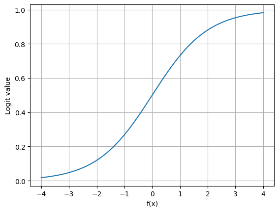
8.14. The Logistic Function#
where
#Sigmoid Function
def logit(fx):
    return np.exp(fx)/(1+np.exp(fx))

fx = np.linspace(-4,4,100)
y = logit(fx)
plt.plot(fx,y)
plt.xlabel('f(x)')
plt.ylabel('Logit value')
plt.grid()
#Dependent categorical variable
y = pd.get_dummies(sba.LoanStatus, dtype=int)
y.head()
| CANCLD | CHGOFF | EXEMPT | PIF | |
|---|---|---|---|---|
| 0 | 1 | 0 | 0 | 0 |
| 1 | 1 | 0 | 0 | 0 |
| 2 | 1 | 0 | 0 | 0 |
| 3 | 0 | 0 | 0 | 1 |
| 4 | 1 | 0 | 0 | 0 |
#Prepare the X and y variables for chargeoffs vs paid in full
idx1 = list(np.where(y.CHGOFF==1)[0])
idx2 = list(np.where(y.PIF==1)[0])
idx = np.append(idx1,idx2)
print(len(idx))
X = X.iloc[idx]
# X["Intercept"] = 1.0

y = y.CHGOFF.iloc[idx]

#Save for later
y_SBA = y.copy()
X_SBA = X.copy()
223647
y_SBA
| CHGOFF | |
|---|---|
| 5 | 1 |
| 8 | 1 |
| 9 | 1 |
| 11 | 1 |
| 14 | 1 |
| ... | ... |
| 508757 | 0 |
| 510524 | 0 |
| 510828 | 0 |
| 511814 | 0 |
| 514919 | 0 |
223647 rows × 1 columns
X_SBA
| ApprovalFiscalYear | InitialInterestRate | TermInMonths | RevolverStatus | JobsSupported | GuaranteePct | 509 - DEALER FLOOR PLAN | Community Advantage Initiative | Community Express | Contract Guaranty | EXPORT IMPORT HARMONIZATION | FA$TRK (Small Loan Express) | Guaranty | Gulf Opportunity | International Trade - Sec, 7(a) (16) | Lender Advantage Initiative | Patriot Express | Revolving Line of Credit Exports - Sec. 7(a) (14) | Rural Lender Advantage | Seasonal Line of Credit | Small Asset Based | Small General Contractors - Sec. 7(a) (9) | Standard Asset Based | CORPORATION | INDIVIDUAL | PARTNERSHIP | |
|---|---|---|---|---|---|---|---|---|---|---|---|---|---|---|---|---|---|---|---|---|---|---|---|---|---|---|
| 5 | 2006 | 11.50 | 28 | 0 | 2 | 0.85 | 0 | 0 | 1 | 0 | 0 | 0 | 0 | 0 | 0 | 0 | 0 | 0 | 0 | 0 | 0 | 0 | 0 | 0 | 1 | 0 |
| 8 | 2006 | 11.25 | 46 | 1 | 6 | 0.50 | 0 | 0 | 0 | 0 | 0 | 1 | 0 | 0 | 0 | 0 | 0 | 0 | 0 | 0 | 0 | 0 | 0 | 1 | 0 | 0 |
| 9 | 2006 | 13.25 | 18 | 0 | 7 | 0.50 | 0 | 0 | 0 | 0 | 0 | 1 | 0 | 0 | 0 | 0 | 0 | 0 | 0 | 0 | 0 | 0 | 0 | 1 | 0 | 0 |
| 11 | 2006 | 12.25 | 32 | 0 | 2 | 0.50 | 0 | 0 | 0 | 0 | 0 | 1 | 0 | 0 | 0 | 0 | 0 | 0 | 0 | 0 | 0 | 0 | 0 | 0 | 1 | 0 |
| 14 | 2006 | 13.25 | 68 | 0 | 1 | 0.50 | 0 | 0 | 0 | 0 | 0 | 1 | 0 | 0 | 0 | 0 | 0 | 0 | 0 | 0 | 0 | 0 | 0 | 1 | 0 | 0 |
| ... | ... | ... | ... | ... | ... | ... | ... | ... | ... | ... | ... | ... | ... | ... | ... | ... | ... | ... | ... | ... | ... | ... | ... | ... | ... | ... |
| 508757 | 2015 | 5.00 | 12 | 1 | 5 | 0.50 | 0 | 0 | 0 | 0 | 0 | 1 | 0 | 0 | 0 | 0 | 0 | 0 | 0 | 0 | 0 | 0 | 0 | 1 | 0 | 0 |
| 510524 | 2015 | 5.50 | 6 | 0 | 0 | 0.50 | 0 | 0 | 0 | 0 | 0 | 1 | 0 | 0 | 0 | 0 | 0 | 0 | 0 | 0 | 0 | 0 | 0 | 1 | 0 | 0 |
| 510828 | 2015 | 6.00 | 60 | 0 | 12 | 0.85 | 0 | 0 | 0 | 0 | 0 | 0 | 0 | 0 | 0 | 1 | 0 | 0 | 0 | 0 | 0 | 0 | 0 | 1 | 0 | 0 |
| 511814 | 2015 | 5.21 | 84 | 0 | 4 | 0.50 | 0 | 0 | 0 | 0 | 0 | 1 | 0 | 0 | 0 | 0 | 0 | 0 | 0 | 0 | 0 | 0 | 0 | 1 | 0 | 0 |
| 514919 | 2015 | 8.75 | 84 | 1 | 0 | 0.50 | 0 | 0 | 0 | 0 | 0 | 1 | 0 | 0 | 0 | 0 | 0 | 0 | 0 | 0 | 0 | 0 | 0 | 0 | 1 | 0 |
223647 rows × 26 columns
%%time

from sklearn.linear_model import LogisticRegression
from sklearn.model_selection import train_test_split
from sklearn.metrics import accuracy_score, roc_auc_score, confusion_matrix, classification_report
from sklearn.model_selection import cross_val_score

# instantiate a logistic regression model, and fit with X and y
model = LogisticRegression(penalty=None, max_iter=1000, tol=0.001) # higher number of iterations needed if the convergence rate is slow
model = model.fit(X, y)

# check the accuracy on the training set
model.score(X, y)
CPU times: user 1min 41s, sys: 331 ms, total: 1min 42s
Wall time: 1min 3s
/usr/local/lib/python3.12/dist-packages/sklearn/linear_model/_logistic.py:465: ConvergenceWarning: lbfgs failed to converge (status=1):
STOP: TOTAL NO. OF ITERATIONS REACHED LIMIT.

Increase the number of iterations (max_iter) or scale the data as shown in:
    https://scikit-learn.org/stable/modules/preprocessing.html
Please also refer to the documentation for alternative solver options:
    https://scikit-learn.org/stable/modules/linear_model.html#logistic-regression
  n_iter_i = _check_optimize_result(
0.8281175244917214
#Show the coefficients
pd.DataFrame({'X':X.columns, 'Coeff':model.coef_[0]})
| X | Coeff | |
|---|---|---|
| 0 | ApprovalFiscalYear | -0.000785 |
| 1 | InitialInterestRate | 0.340614 |
| 2 | TermInMonths | -0.043086 |
| 3 | RevolverStatus | -0.372911 |
| 4 | JobsSupported | -0.000131 |
| 5 | GuaranteePct | -0.147432 |
| 6 | 509 - DEALER FLOOR PLAN | -0.054297 |
| 7 | Community Advantage Initiative | -0.008525 |
| 8 | Community Express | 1.519302 |
| 9 | Contract Guaranty | -0.306267 |
| 10 | EXPORT IMPORT HARMONIZATION | -0.027176 |
| 11 | FA$TRK (Small Loan Express) | -0.066487 |
| 12 | Guaranty | 1.621458 |
| 13 | Gulf Opportunity | -1.235105 |
| 14 | International Trade - Sec, 7(a) (16) | -0.009399 |
| 15 | Lender Advantage Initiative | -0.476701 |
| 16 | Patriot Express | 1.528784 |
| 17 | Revolving Line of Credit Exports - Sec. 7(a) (14) | -1.668423 |
| 18 | Rural Lender Advantage | -0.064062 |
| 19 | Seasonal Line of Credit | -0.048712 |
| 20 | Small Asset Based | -0.037235 |
| 21 | Small General Contractors - Sec. 7(a) (9) | -0.133957 |
| 22 | Standard Asset Based | -0.503938 |
| 23 | CORPORATION | 0.156950 |
| 24 | INDIVIDUAL | 0.177251 |
| 25 | PARTNERSHIP | -0.303480 |
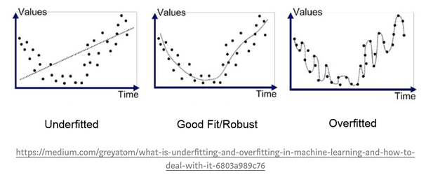
8.15. Training, validation, and testing data: Underfitting, Overfitting, Cross-Validation#
As we will see below, we split our data sample into training and testing subsets. Training data is used for machine learning a model and then the same model is applied to the test data (out-of-sample) to make sure the model performs well on data it has not already seen. The same model is also applied back to the same data on which it was trained. So, we get two accuracy scores, one on the training data set and another for the test data set. One hopes that a model performs as accurately on the test data as it does on the training data.
When accuracy is low on the training data, the model “underfits” the data. However, it may show a very high level of accuracy on the training data. This is a good thing, unless it achieves a very low accuracy level on the test data. In this case, we say that the model is “overfitted” to the data. The model is too specifically attuned to the training data so that it is useless for data outside the training data set. This occurs when the model has too many free parameters so it almost “memorizes” the training data set, which explains why it performs poorly on data it has not seen before. An analogy to this occurs when students memorize math homework problems without understanding the underlying concepts. When faced with a slightly different problem on the exam, they fail miserably.
We often break down a data sample into 3 types of data: training, validation, and testing data. Say we keep 20% of our data aside for testing. This is also known as “holdout” data. Of the remaining 80% data we may randomly sample 75% of it, and train the model so that it performs well on the remaining 25%. Then we randomly sample a different 75% and train to fit the remaining 25% starting from the current model or afresh. This is also called “rotation sampling”. If we repeat this \(n\) times to get the best model, we are said to undertake “\(n\)-fold cross-validation”. The results are averaged to assess fit. Once a model has been trained through this cross-validated process, it is then taken to the test data to assess how well it performs and determination is made as to the extent of overfitting, if any.
The figure below provides a visual depiction of under- and over-fitting.
Image("NLP_images/overfitting.png", width=1000)
# Evaluate the model by splitting into train and test sets
X_train, X_test, y_train, y_test = train_test_split(X, y, test_size=0.3, random_state=0)
model2 = LogisticRegression(penalty=None, max_iter=1000, tol=0.001)
model2.fit(X_train, y_train)
LogisticRegression(max_iter=1000, penalty=None, tol=0.001)In a Jupyter environment, please rerun this cell to show the HTML representation or trust the notebook.
On GitHub, the HTML representation is unable to render, please try loading this page with nbviewer.org.
LogisticRegression(max_iter=1000, penalty=None, tol=0.001)
# Predict class labels for the test set
predicted = model2.predict(X_test)
print(predicted)
[0 0 0 ... 1 1 1]
# Generate class probabilities
probs = model2.predict_proba(X_test)
print(probs)
[[0.93025884 0.06974116]
 [0.95258196 0.04741804]
 [0.83374884 0.16625116]
 ...
 [0.29915793 0.70084207]
 [0.41565239 0.58434761]
 [0.22631199 0.77368801]]
model2.score(X_test, y_test)
0.8289589388180938
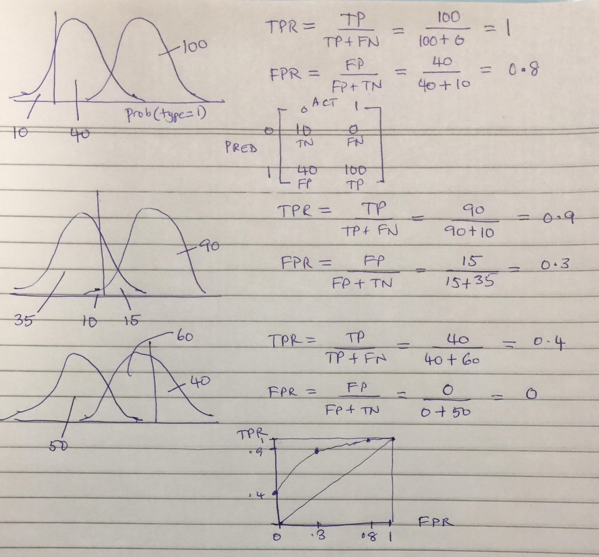
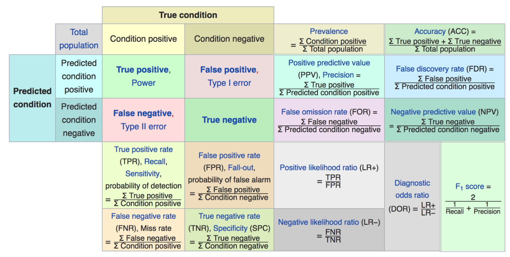
8.16. Metrics#
Accuracy: the number of correctly predicted class values.
TPR = sensitivity or recall = TP/(TP+FN)
FPR = (1 − specificity) = FP/(FP+TN)
# Confusion Matrix
CM = confusion_matrix(predicted, y_test) # predicted values on rows, true values on columns
CM
array([[43703,  7991],
       [ 3485, 11916]])
8.17. More Metrics#
Precision = \(\frac{TP}{TP+FP}\)
Recall = \(\frac{TP}{TP+FN}\)
F1 score = \(\frac{2}{\frac{1}{Precision} + \frac{1}{Recall}}\)
(F1 is the harmonic mean of precision and recall.)
print(classification_report(predicted, y_test))
              precision    recall  f1-score   support

           0       0.93      0.85      0.88     51694
           1       0.60      0.77      0.67     15401

    accuracy                           0.83     67095
   macro avg       0.76      0.81      0.78     67095
weighted avg       0.85      0.83      0.84     67095
8.18. The Matthews Correlation Coefficient#
https://en.wikipedia.org/wiki/Matthews_correlation_coefficient
This is a useful classification metric that is not widely used. See: https://towardsdatascience.com/the-best-classification-metric-youve-never-heard-of-the-matthews-correlation-coefficient-3bf50a2f3e9a
def MCC(tp,tn,fp,fn):
  return (tp*tn - fp*fn)/np.sqrt((tp+fp)*(tp+fn)*(tn+fp)*(tn+fn))
Let’s take the confusion matrix from above and apply the numbers therein to compute MCC.
print(CM)
mcc = MCC(CM[1,1], CM[0,0], CM[0,1], CM[1,0])
print("MCC =", mcc)
[[43703  7991]
 [ 3485 11916]]
MCC = 0.5699804607095624
8.19. ROC and AUC#
The Receiver-Operating Characteristic (ROC) curve is a plot of the True Positive Rate (TPR) against the False Positive Rate (FPR) for different levels of the cut-off posterior probability. This is an essential trade-off in all classification systems.
Image("NLP_images/roc_example.jpg", width=600)
# generate evaluation metrics
print('Accuracy =', accuracy_score(y_test, predicted))
print('AUC =', roc_auc_score(y_test, probs[:, 1]))
Accuracy = 0.8289589388180938
AUC = 0.8634186497943588
#ROC, AUC
from sklearn.metrics import roc_curve, auc
y_score = model.predict_proba(X_test)[:,1]
fpr, tpr, _ = roc_curve(y_test, y_score)

plt.title('ROC curve')
plt.xlabel('FPR (Precision)')
plt.ylabel('TPR (Recall)')

plt.plot(fpr,tpr)
plt.plot((0,1), ls='dashed',color='black')
plt.show()
print('Area under curve (AUC): ', auc(fpr,tpr))
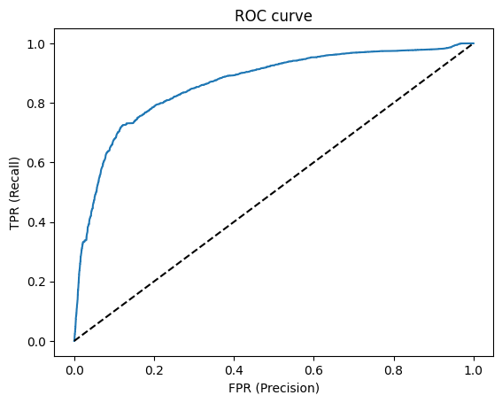
Area under curve (AUC): 0.863236455638921
8.20. All In One#
A terrific article in Scientific American on ROC Curves by Swets, Dawes, Monahan (2000); pdf. And Dawes (1979) on the use of “Improper Linear Models”.
https://en.wikipedia.org/wiki/Receiver_operating_characteristic
Image("NLP_images/all_metrics.png", width=800)
8.21. ML Comic#
Google has put out an interesting comic book introduction to Machine Learning; pdf.
For a visual understanding of many ML concepts, Amazon has created https://www.amazon.science/latest-news/amazon-machine-learning-university-new-courses-mlu-explains