
28. Topic Modeling#
Extracting topics from a collection of documents.
from google.colab import drive
drive.mount('/content/drive')  # Add My Drive/<>

import os
os.chdir('drive/My Drive')
os.chdir('Books_Writings/NLPBook/')
Mounted at /content/drive
%%capture
%pylab inline
import pandas as pd
import os
%load_ext rpy2.ipython
from IPython.display import Image
28.1. Topic Modeling using LDA#
This is a nice article that has most of what is needed: https://www.analyticsvidhya.com/blog/2016/08/beginners-guide-to-topic-modeling-in-python/
28.2. LDA Explained (Briefly)#
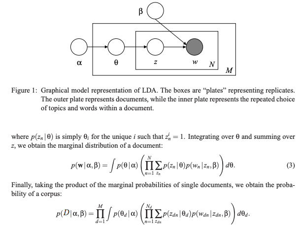
Latent Dirichlet Allocation (LDA) was created by David Blei, Andrew Ng, and Michael Jordan in 2003, see their paper titled “Latent Dirichlet Allocation” in the Journal of Machine Learning Research, pp 993–1022: http://www.jmlr.org/papers/volume3/blei03a/blei03a.pdf
The simplest way to think about LDA is as a probability model that connects documents with words and topics. The components are:
A Vocabulary of \(V\) words, i.e., \(w_1,w_2,...,w_i,...,w_V\), each word indexed by \(i\).
A Document is a vector of \(N\) words, i.e., \({\bf w}\).
A Corpus \(D\) is a collection of \(M\) documents, each document indexed by \(j\), i.e. \(d_j\).
Next, we connect the above objects to \(K\) topics, indexed by \(l\), i.e., \(t_l\). We will see that LDA is encapsulated (conceptually) in two matrices: Matrix \(A\) and Matrix \(B\).
## LDA Decomposition

Image('NLP_images/LDA_decomp.png', width=800)
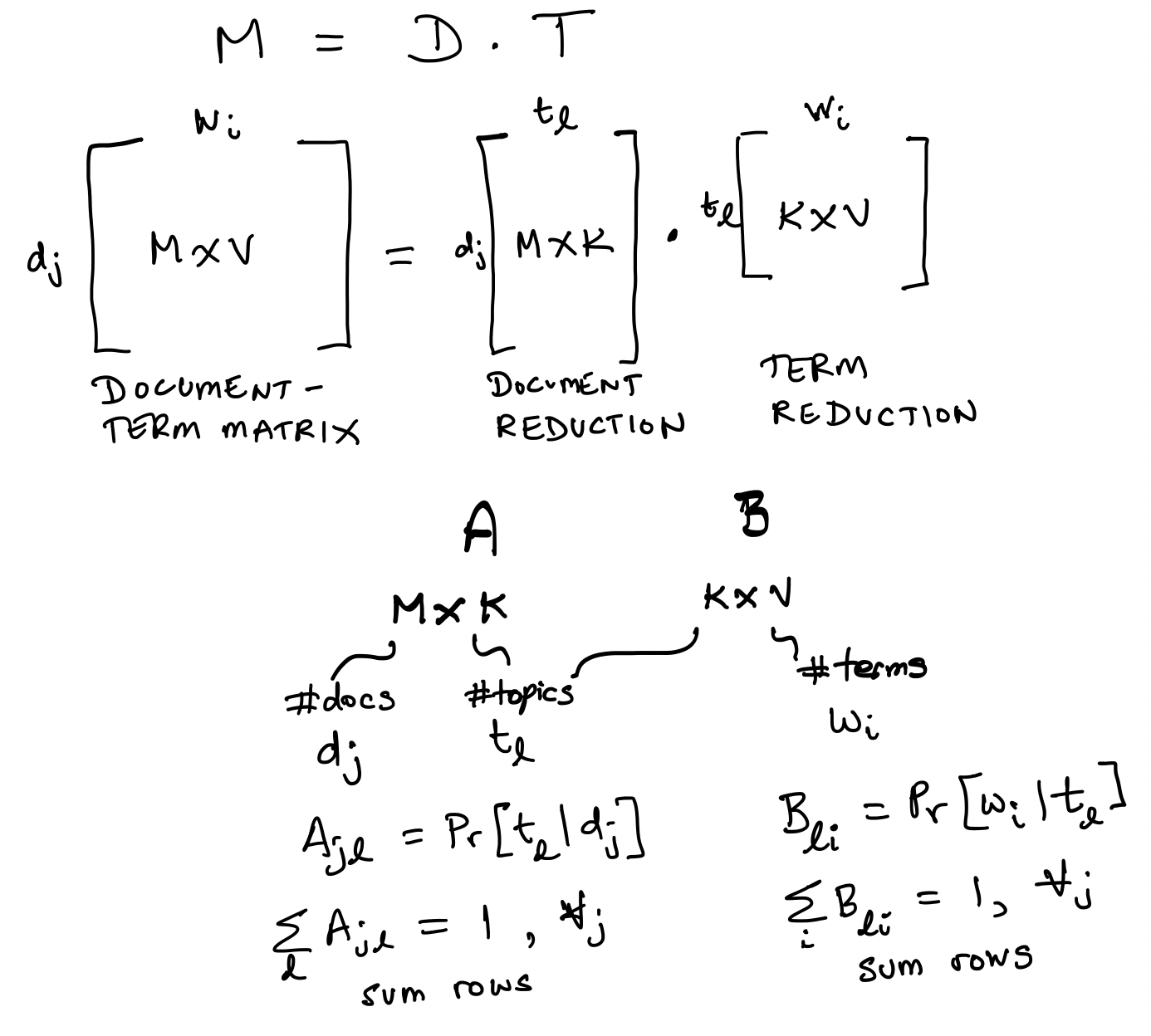
28.3. Matrix \(A\): Connecting Documents with Topics#
This matrix has documents on the rows, so there are \(M\) rows.
The topics are on the columns, so there are \(K\) columns.
Therefore \(A \in {R}^{M \times K}\).
The row sums equal \(1\), i.e., for each document, we have a probability that it pertains to a given topic, i.e., \(A_{jl} = Pr[t_l | d_j]\), and \(\sum_{l=1}^K A_{jl} = 1\).
28.4. Matrix \(B\): Connecting Words with Topics#
This matrix has topics on the rows, so there are \(K\) rows.
The words are on the columns, so there are \(V\) columns.
Therefore \(B \in {R}^{K \times V}\).
The row sums equal \(1\), i.e., for each topic, we have a probability that it pertains to a given word, i.e., \(B_{li} = Pr[w_i | t_l]\), and \(\sum_{i=1}^V B_{li} = 1\).
28.5. Distribution of Topics in a Document#
This is a generative model, i.e., we have a prior on topics in documents from which we sample to create a topic vector with probabilities of dimension \(K\), adding up to 1. (Compare this to discriminative models.)
Using Matrix \(A\), we can sample a \(K\)-vector of probabilities of topics for a single document. Denote the probability of this vector as \(p(\theta | \alpha)\), where \(\theta, \alpha \in {R}^K\), \(\theta, \alpha \geq 0\), and \(\sum_l \theta_l = 1\).
The probability \(p(\theta | \alpha)\) is governed by a Dirichlet distribution, with density function
where \(\Gamma(\cdot)\) is the Gamma function.
LDA thus gets its name from the use of the Dirichlet distribution, embodied in Matrix \(A\). Since the topics are latent, it explains the rest of the nomenclature.
Given \(\theta\), we sample topics from matrix \(A\) with probability \(p(t | \theta)\).
Note: https://en.wikipedia.org/wiki/Dirichlet_distribution
# Dirichlet Basics
alpha = rand(5) # concentration parameters
print("alpha=",alpha)
theta = array([0.1,0.2,0.4,0.2,0.1])  # topic mixture

from scipy.stats import dirichlet
print("PDF of theta =",dirichlet.pdf(theta, alpha))
print("Draw a random theta =",dirichlet.rvs(alpha).round(2))
alpha= [0.37137576 0.02668608 0.60548522 0.72547081 0.04330351]
PDF of theta = 0.1025913793533479
Draw a random theta = [[0.01 0.   0.4  0.59 0.01]]
28.6. Distribution of Words and Topics for a Document#
And then, a generative model for words.
The number of words in a document is assumed to be distributed Poisson with parameter \(\xi\).
Matrix \(B\) gives the multinomial probability of a word appearing in a topic, \(p(w | t)\).
The topics mixture is given by \(\theta\).
The joint distribution over \(K\) topics and \(K\) words for a topic mixture is given by
The marginal distribution for a document’s words comes from integrating out the topic mixture \(\theta\), and summing out the topics \({\bf t}\), i.e.,
28.7. Likelihood of the entire Corpus#
This is given by:
The goal is to maximize this likelihood by picking the vector \(\alpha\) and the probabilities in the matrix \(B\). (Note that were a Dirichlet distribution not used, then we could directly pick values in Matrices \(A\) and \(B\).)
The computation is undertaken using MCMC with Gibbs sampling.
## Recap LDA

Image('NLP_images/LDA_diagram.png', width=800)
28.8. Load in the Reuters news corpus#
This data can be obtained here: https://raw.githubusercontent.com/nltk/nltk_data/gh-pages/packages/corpora/reuters.zip
Please drop it into the folder NLP_data, using the directory structure shown below. Or just use the code in the next block to download the data and place it in the folder NLP_data/reuters/.
Run this block only once to get the data. You do not need to re-run it once you have the news articles in your file system.
%%time
os.system('wget https://raw.githubusercontent.com/nltk/nltk_data/gh-pages/packages/corpora/reuters.zip')
os.system('mv reuters.zip NLP_data/')
os.system('unzip NLP_data/reuters.zip')
os.system('mv reuters/ NLP_data/')
os.system('rm NLP_data/reuters.zip')
CPU times: user 4.67 ms, sys: 1.5 ms, total: 6.17 ms
Wall time: 2min 26s
0
28.9. Text Cleaning Functions#
Simple functions to remove numbers, punctuation, stopwords, and undertake stemming. We will use these to prepare the news articles downloaded above from Reuters.
import nltk

# Remove punctuations
import string
def removePuncStr(s):
    for c in string.punctuation:
        s = s.replace(c," ")
    return s

def removePunc(text_array):
    return [removePuncStr(h) for h in text_array]

# Remove numbers
def removeNumbersStr(s):
    for c in range(10):
        n = str(c)
        s = s.replace(n," ")
    return s

def removeNumbers(text_array):
    return [removeNumbersStr(h) for h in text_array]

# Stemming
nltk.download('punkt')
from nltk.stem import PorterStemmer
from nltk.tokenize import sent_tokenize, word_tokenize

def stemText(text_array):
    stemmed_text = []
    for h in text_array:
        words = word_tokenize(h)
        h2 = ''
        for w in words:
            h2 = h2 + ' ' + PorterStemmer().stem(w)
        stemmed_text.append(h2)
    return stemmed_text

# Remove Stopwords
nltk.download('stopwords')
from nltk.corpus import stopwords
from nltk.tokenize import word_tokenize

def stopText(text_array):
    stop_words = set(stopwords.words('english'))
    stopped_text = []
    for h in text_array:
        words = word_tokenize(h)
        h2 = ''
        for w in words:
            if w not in stop_words:
                h2 = h2 + ' ' + w
        stopped_text.append(h2)
    return stopped_text

# Write all docs to separate files
def write2textfile(s,filename):
    text_file = open(filename, "w")
    text_file.write(s)
    text_file.close()
[nltk_data] Downloading package punkt to /root/nltk_data...
[nltk_data]   Unzipping tokenizers/punkt.zip.
[nltk_data] Downloading package stopwords to /root/nltk_data...
[nltk_data]   Unzipping corpora/stopwords.zip.
#Read in the corpus
from nltk.corpus import PlaintextCorpusReader
corpus_root = 'NLP_data/reuters/training/'
ctext = PlaintextCorpusReader(corpus_root, '.*')
%%time
# Corpus Statistics
import nltk
nltk.download('punkt_tab')
print(len(ctext.fileids()))
print(len(ctext.paras()))
print(len(ctext.sents()))
print(len(ctext.words()))
print(len(ctext.raw()))
[nltk_data] Downloading package punkt_tab to /root/nltk_data...
[nltk_data]   Unzipping tokenizers/punkt_tab.zip.
7769
8471
40277
1253696
6478471
CPU times: user 14.1 s, sys: 7.36 s, total: 21.4 s
Wall time: 3min 34s
#Convert corpus to text array with a full string for each doc
def merge_arrays(word_lists):
    wordlist = []
    for wl in word_lists:
        wordlist = wordlist + wl
    doc = ' '.join(wordlist)
    return doc
#Run this through the corpus to get a word array for each doc
text_array = []
for p in ctext.paras():
    doc = merge_arrays(p)
    text_array.append(doc)

#Clean up the docs using the previous functions
news = text_array
news = removePunc(news)
news = removeNumbers(news)
news = stopText(news)
#news = stemText(news)
news = [j.lower() for j in news]
news[:2]
[' bahia cocoa review showers continued throughout week bahia cocoa zone alleviating drought since early january improving prospects coming temporao although normal humidity levels restored comissaria smith said weekly review the dry period means temporao late year arrivals week ended february bags kilos making cumulative total season mln stage last year again seems cocoa delivered earlier consignment included arrivals figures comissaria smith said still doubt much old crop cocoa still available harvesting practically come end with total bahia crop estimates around mln bags sales standing almost mln hundred thousand bags still hands farmers middlemen exporters processors there doubts much cocoa would fit export shippers experiencing dificulties obtaining bahia superior certificates in view lower quality recent weeks farmers sold good part cocoa held consignment comissaria smith said spot bean prices rose cruzados per arroba kilos bean shippers reluctant offer nearby shipment limited sales booked march shipment dlrs per tonne ports named new crop sales also light open ports june july going dlrs dlrs new york july aug sept dlrs per tonne fob routine sales butter made march april sold dlrs april may butter went times new york may june july dlrs aug sept dlrs times new york sept oct dec dlrs times new york dec comissaria smith said destinations u s covertible currency areas uruguay open ports cake sales registered dlrs march april dlrs may dlrs aug times new york dec oct dec buyers u s argentina uruguay convertible currency areas liquor sales limited march april selling dlrs june july dlrs times new york july aug sept dlrs times new york sept oct dec times new york dec comissaria smith said total bahia sales currently estimated mln bags crop mln bags crop final figures period february expected published brazilian cocoa trade commission carnival ends midday february',
 ' computer terminal systems lt cpml completes sale computer terminal systems inc said completed sale shares common stock warrants acquire additional one mln shares lt sedio n v lugano switzerland dlrs the company said warrants exercisable five years purchase price dlrs per share computer terminal said sedio also right buy additional shares increase total holdings pct computer terminal outstanding common stock certain circumstances involving change control company the company said conditions occur warrants would exercisable price equal pct common stock market price time exceed dlrs per share computer terminal also said sold technolgy rights dot matrix impact technology including future improvements lt woodco inc houston tex dlrs but said would continue exclusive worldwide licensee technology woodco the company said moves part reorganization plan would help pay current operation costs ensure product delivery computer terminal makes computer generated labels forms tags ticket printers terminals']
28.10. Lemmatization#
Stemming reduces words to their root form. The root form may not be an actual word in the language being processed. The goal of stemming is to reduce the number of forms of the word to a single form, so that when the term-document matrix is constructed, the same word does not appear as different words, as it may conflate the textual analysis being undertaken.
Stemming is a hard problem and a long-standing solution was developed by Porter in 1979. This has stood the test of time. https://tartarus.org/martin/PorterStemmer/. The Lancaster stemmer is more aggressive and was developed in 1990, the source code is quite economical and you can see it here: https://www.nltk.org/_modules/nltk/stem/lancaster.html
Lemmatization is the same as stemming with the additional constraint that the root word is present in the language’s dictionary. NLTK uses the WordNet lemmatizer. (WordNet is a widely used word corpus also known as a “lexical database”.) See: https://wordnet.princeton.edu/
Additional reading: https://www.datacamp.com/community/tutorials/stemming-lemmatization-python
nltk.download('wordnet')
nltk.download('omw-1.4')
from nltk.stem import WordNetLemmatizer
from nltk.tokenize import sent_tokenize, word_tokenize

def lemmText(text_array):
    WNlemmatizer = WordNetLemmatizer()
    lemmatized_text = []
    for h in text_array:
        words = word_tokenize(h)
        h2 = ''
        for w in words:
            h2 = h2 + ' ' + WNlemmatizer.lemmatize(w)
        lemmatized_text.append(h2)
    return lemmatized_text
[nltk_data] Downloading package wordnet to /root/nltk_data...
[nltk_data] Downloading package omw-1.4 to /root/nltk_data...
#Example
import textwrap

bio = [' Citibank His current research interests include machine learning',
       ' social networks derivatives pricing models portfolio theory',
       ' modeling default risk systemic risk venture capital He',
       ' published hundred articles academic journals',
       ' numerous awards research teaching His recent book',
       ' Derivatives Principles Practice published May second edition']
temp = stopText(removeNumbers(removePunc(bio)))
print('Original: ',temp, "\n")
bio_lemm = lemmText(temp)
print('Lemmatized: ',bio_lemm, "\n")
bio_stem = stemText(temp)
print('Stemmed: ',bio_stem)
Original:  [' Citibank His current research interests include machine learning', ' social networks derivatives pricing models portfolio theory', ' modeling default risk systemic risk venture capital He', ' published hundred articles academic journals', ' numerous awards research teaching His recent book', ' Derivatives Principles Practice published May second edition']

Lemmatized:  [' Citibank His current research interest include machine learning', ' social network derivative pricing model portfolio theory', ' modeling default risk systemic risk venture capital He', ' published hundred article academic journal', ' numerous award research teaching His recent book', ' Derivatives Principles Practice published May second edition']

Stemmed:  [' citibank hi current research interest includ machin learn', ' social network deriv price model portfolio theori', ' model default risk system risk ventur capit he', ' publish hundr articl academ journal', ' numer award research teach hi recent book', ' deriv principl practic publish may second edit']
#Clean and process news documents into shape for LDA
from nltk.corpus import stopwords
from nltk.stem.wordnet import WordNetLemmatizer
import string

stop = set(stopwords.words('english'))
exclude = set(string.punctuation)
lemma = WordNetLemmatizer()
def clean(doc):
    stop_free = " ".join([i for i in doc.lower().split() if i not in stop])
    punc_free = ''.join(ch for ch in stop_free if ch not in exclude)
    normalized = " ".join(lemma.lemmatize(word) for word in punc_free.split())
    return normalized

doc_clean = [clean(doc).split() for doc in news]
print(len(doc_clean))
type(doc_clean)
8471
list
for j in range(5):
    print(doc_clean[j])
['bahia', 'cocoa', 'review', 'shower', 'continued', 'throughout', 'week', 'bahia', 'cocoa', 'zone', 'alleviating', 'drought', 'since', 'early', 'january', 'improving', 'prospect', 'coming', 'temporao', 'although', 'normal', 'humidity', 'level', 'restored', 'comissaria', 'smith', 'said', 'weekly', 'review', 'dry', 'period', 'mean', 'temporao', 'late', 'year', 'arrival', 'week', 'ended', 'february', 'bag', 'kilo', 'making', 'cumulative', 'total', 'season', 'mln', 'stage', 'last', 'year', 'seems', 'cocoa', 'delivered', 'earlier', 'consignment', 'included', 'arrival', 'figure', 'comissaria', 'smith', 'said', 'still', 'doubt', 'much', 'old', 'crop', 'cocoa', 'still', 'available', 'harvesting', 'practically', 'come', 'end', 'total', 'bahia', 'crop', 'estimate', 'around', 'mln', 'bag', 'sale', 'standing', 'almost', 'mln', 'hundred', 'thousand', 'bag', 'still', 'hand', 'farmer', 'middleman', 'exporter', 'processor', 'doubt', 'much', 'cocoa', 'would', 'fit', 'export', 'shipper', 'experiencing', 'dificulties', 'obtaining', 'bahia', 'superior', 'certificate', 'view', 'lower', 'quality', 'recent', 'week', 'farmer', 'sold', 'good', 'part', 'cocoa', 'held', 'consignment', 'comissaria', 'smith', 'said', 'spot', 'bean', 'price', 'rose', 'cruzados', 'per', 'arroba', 'kilo', 'bean', 'shipper', 'reluctant', 'offer', 'nearby', 'shipment', 'limited', 'sale', 'booked', 'march', 'shipment', 'dlrs', 'per', 'tonne', 'port', 'named', 'new', 'crop', 'sale', 'also', 'light', 'open', 'port', 'june', 'july', 'going', 'dlrs', 'dlrs', 'new', 'york', 'july', 'aug', 'sept', 'dlrs', 'per', 'tonne', 'fob', 'routine', 'sale', 'butter', 'made', 'march', 'april', 'sold', 'dlrs', 'april', 'may', 'butter', 'went', 'time', 'new', 'york', 'may', 'june', 'july', 'dlrs', 'aug', 'sept', 'dlrs', 'time', 'new', 'york', 'sept', 'oct', 'dec', 'dlrs', 'time', 'new', 'york', 'dec', 'comissaria', 'smith', 'said', 'destination', 'u', 'covertible', 'currency', 'area', 'uruguay', 'open', 'port', 'cake', 'sale', 'registered', 'dlrs', 'march', 'april', 'dlrs', 'may', 'dlrs', 'aug', 'time', 'new', 'york', 'dec', 'oct', 'dec', 'buyer', 'u', 'argentina', 'uruguay', 'convertible', 'currency', 'area', 'liquor', 'sale', 'limited', 'march', 'april', 'selling', 'dlrs', 'june', 'july', 'dlrs', 'time', 'new', 'york', 'july', 'aug', 'sept', 'dlrs', 'time', 'new', 'york', 'sept', 'oct', 'dec', 'time', 'new', 'york', 'dec', 'comissaria', 'smith', 'said', 'total', 'bahia', 'sale', 'currently', 'estimated', 'mln', 'bag', 'crop', 'mln', 'bag', 'crop', 'final', 'figure', 'period', 'february', 'expected', 'published', 'brazilian', 'cocoa', 'trade', 'commission', 'carnival', 'end', 'midday', 'february']
['computer', 'terminal', 'system', 'lt', 'cpml', 'completes', 'sale', 'computer', 'terminal', 'system', 'inc', 'said', 'completed', 'sale', 'share', 'common', 'stock', 'warrant', 'acquire', 'additional', 'one', 'mln', 'share', 'lt', 'sedio', 'n', 'v', 'lugano', 'switzerland', 'dlrs', 'company', 'said', 'warrant', 'exercisable', 'five', 'year', 'purchase', 'price', 'dlrs', 'per', 'share', 'computer', 'terminal', 'said', 'sedio', 'also', 'right', 'buy', 'additional', 'share', 'increase', 'total', 'holding', 'pct', 'computer', 'terminal', 'outstanding', 'common', 'stock', 'certain', 'circumstance', 'involving', 'change', 'control', 'company', 'company', 'said', 'condition', 'occur', 'warrant', 'would', 'exercisable', 'price', 'equal', 'pct', 'common', 'stock', 'market', 'price', 'time', 'exceed', 'dlrs', 'per', 'share', 'computer', 'terminal', 'also', 'said', 'sold', 'technolgy', 'right', 'dot', 'matrix', 'impact', 'technology', 'including', 'future', 'improvement', 'lt', 'woodco', 'inc', 'houston', 'tex', 'dlrs', 'said', 'would', 'continue', 'exclusive', 'worldwide', 'licensee', 'technology', 'woodco', 'company', 'said', 'move', 'part', 'reorganization', 'plan', 'would', 'help', 'pay', 'current', 'operation', 'cost', 'ensure', 'product', 'delivery', 'computer', 'terminal', 'make', 'computer', 'generated', 'label', 'form', 'tag', 'ticket', 'printer', 'terminal']
['n', 'z', 'trading', 'bank', 'deposit', 'growth', 'rise', 'slightly', 'new', 'zealand', 'trading', 'bank', 'seasonally', 'adjusted', 'deposit', 'growth', 'rose', 'pct', 'january', 'compared', 'rise', 'pct', 'december', 'reserve', 'bank', 'said', 'year', 'year', 'total', 'deposit', 'rose', 'pct', 'compared', 'pct', 'increase', 'december', 'year', 'pct', 'rise', 'year', 'ago', 'period', 'said', 'weekly', 'statistical', 'release', 'total', 'deposit', 'rose', 'billion', 'n', 'z', 'dlrs', 'january', 'compared', 'billion', 'december', 'billion', 'january']
['national', 'amusement', 'ups', 'viacom', 'lt', 'via', 'bid', 'viacom', 'international', 'inc', 'said', 'lt', 'national', 'amusement', 'inc', 'raised', 'value', 'offer', 'viacom', 'publicly', 'held', 'stock', 'company', 'said', 'special', 'committee', 'board', 'plan', 'meet', 'later', 'today', 'consider', 'offer', 'one', 'submitted', 'march', 'one', 'lt', 'mcv', 'holding', 'inc', 'spokeswoman', 'unable', 'say', 'committee', 'met', 'planned', 'yesterday', 'viacom', 'said', 'national', 'amusement', 'arsenal', 'holding', 'inc', 'subsidiary', 'raised', 'amount', 'cash', 'offering', 'viacom', 'share', 'ct', 'dlrs', 'value', 'fraction', 'share', 'exchangeable', 'arsenal', 'holding', 'preferred', 'included', 'raised', 'ct', 'dlrs', 'national', 'amusement', 'already', 'owns', 'pct', 'viacom', 'stock']
['rogers', 'lt', 'rog', 'see', 'st', 'qtr', 'net', 'significantly', 'rogers', 'corp', 'said', 'first', 'quarter', 'earnings', 'significantly', 'earnings', 'dlrs', 'four', 'ct', 'share', 'quarter', 'last', 'year', 'company', 'said', 'expects', 'revenue', 'first', 'quarter', 'somewhat', 'higher', 'revenue', 'mln', 'dlrs', 'posted', 'year', 'ago', 'quarter', 'rogers', 'said', 'reached', 'agreement', 'sale', 'molded', 'switch', 'circuit', 'product', 'line', 'major', 'supplier', 'sale', 'term', 'disclosed', 'completed', 'early', 'second', 'quarter', 'rogers', 'said']
28.11. Gensim for topic analysis#
Stands for “generate similar”.
https://radimrehurek.com/gensim/
There are several useful tutorials in this site. we will run the algorithm first and then discuss further two approaches for topic modeling.
!pip install --upgrade smart_open
!pip install --upgrade gensim
Requirement already satisfied: smart_open in /usr/local/lib/python3.12/dist-packages (7.4.1)
Collecting smart_open
  Downloading smart_open-7.4.4-py3-none-any.whl.metadata (24 kB)
Requirement already satisfied: wrapt in /usr/local/lib/python3.12/dist-packages (from smart_open) (2.0.0)
Downloading smart_open-7.4.4-py3-none-any.whl (63 kB)
   ━━━━━━━━━━━━━━━━━━━━━━━━━━━━━━━━━━━━━━━━ 63.0/63.0 kB 2.2 MB/s eta 0:00:00
?25hInstalling collected packages: smart_open
  Attempting uninstall: smart_open
    Found existing installation: smart_open 7.4.1
    Uninstalling smart_open-7.4.1:
      Successfully uninstalled smart_open-7.4.1
Successfully installed smart_open-7.4.4
Collecting gensim
  Downloading gensim-4.4.0-cp312-cp312-manylinux_2_24_x86_64.manylinux_2_28_x86_64.whl.metadata (8.4 kB)
Requirement already satisfied: numpy>=1.18.5 in /usr/local/lib/python3.12/dist-packages (from gensim) (2.0.2)
Requirement already satisfied: scipy>=1.7.0 in /usr/local/lib/python3.12/dist-packages (from gensim) (1.16.3)
Requirement already satisfied: smart_open>=1.8.1 in /usr/local/lib/python3.12/dist-packages (from gensim) (7.4.4)
Requirement already satisfied: wrapt in /usr/local/lib/python3.12/dist-packages (from smart_open>=1.8.1->gensim) (2.0.0)
Downloading gensim-4.4.0-cp312-cp312-manylinux_2_24_x86_64.manylinux_2_28_x86_64.whl (27.9 MB)
   ━━━━━━━━━━━━━━━━━━━━━━━━━━━━━━━━━━━━━━━━ 27.9/27.9 MB 14.8 MB/s eta 0:00:00
?25hInstalling collected packages: gensim
Successfully installed gensim-4.4.0
# Importing Gensim
import gensim
from gensim import corpora

# Creating the term dictionary of our corpus, every unique term is assigned an index.
dictionary = corpora.Dictionary(doc_clean)

# Converting list of documents (corpus) into Document Term Matrix using dictionary above.
doc_term_matrix = [dictionary.doc2bow(doc) for doc in doc_clean]
print(len(doc_term_matrix))
print(type(doc_term_matrix))
print(len(doc_term_matrix[0]))
print(len(doc_term_matrix[1]))
8471
<class 'list'>
149
86
%%time
#RUN THE MODEL
# Creating the object for LDA model using gensim library
Lda = gensim.models.ldamodel.LdaModel

# Running and Training LDA model on the document term matrix.
ldamodel = Lda(doc_term_matrix, num_topics=3, id2word = dictionary, passes=50)
CPU times: user 2min 27s, sys: 178 ms, total: 2min 27s
Wall time: 2min 38s
#Results
print(ldamodel.print_topics(num_topics=3, num_words=25))
[(0, '0.029*"said" + 0.023*"pct" + 0.016*"mln" + 0.016*"billion" + 0.015*"year" + 0.014*"bank" + 0.010*"u" + 0.009*"rate" + 0.008*"market" + 0.008*"tonne" + 0.008*"dlrs" + 0.007*"january" + 0.006*"february" + 0.006*"last" + 0.006*"dollar" + 0.005*"trade" + 0.005*"price" + 0.005*"rise" + 0.005*"month" + 0.005*"export" + 0.005*"rose" + 0.004*"week" + 0.004*"mark" + 0.004*"would" + 0.004*"stg"'), (1, '0.052*"mln" + 0.052*"v" + 0.034*"dlrs" + 0.033*"ct" + 0.029*"lt" + 0.026*"net" + 0.024*"loss" + 0.019*"share" + 0.015*"shr" + 0.015*"profit" + 0.014*"said" + 0.014*"year" + 0.014*"inc" + 0.012*"company" + 0.011*"corp" + 0.010*"sale" + 0.009*"qtr" + 0.009*"rev" + 0.006*"note" + 0.006*"stock" + 0.006*"dividend" + 0.005*"april" + 0.005*"co" + 0.005*"oper" + 0.005*"pct"'), (2, '0.038*"said" + 0.010*"u" + 0.010*"would" + 0.008*"company" + 0.008*"oil" + 0.006*"price" + 0.005*"offer" + 0.005*"trade" + 0.005*"new" + 0.004*"pct" + 0.004*"lt" + 0.004*"stock" + 0.004*"agreement" + 0.004*"also" + 0.004*"dlrs" + 0.004*"state" + 0.003*"share" + 0.003*"market" + 0.003*"group" + 0.003*"last" + 0.003*"official" + 0.003*"industry" + 0.003*"one" + 0.003*"told" + 0.003*"plan"')]
28.12. Two approaches to topic modeling:#
[1] Latent Semantic Analysis (LSA): implements a matrix decomposition of the DTM \(M\) into a \(D\) matrix and an \(T\), by minimizing the Frobenious norm, i.e.,
Implemented with a truncated SVD.
[2] LDA: Latent Dirichlet Allocation (discussed above)
28.13. LSA : Latent Semantic Analysis#
See Linear Algebra Notebook 2: 022-LinearAlgebra_Eigensystems_Decompositions
https://srdas.github.io/MLBook2/24_TextAnaytics_Advanced.html#Singular-Value-Decomposition-(SVD)
See R code below.
%%R
system("mkdir D")
write( c("blue", "red", "green"), file=paste("D", "D1.txt", sep="/"))
write( c("black", "blue", "red"), file=paste("D", "D2.txt", sep="/"))
write( c("yellow", "black", "green"), file=paste("D", "D3.txt", sep="/"))
write( c("yellow", "red", "black"), file=paste("D", "D4.txt", sep="/"))
%%R
install.packages("lsa", quiet=TRUE)
also installing the dependency ‘SnowballC’
%%R
library(lsa)
tdm = textmatrix("D",minWordLength=1)
print(tdm)
system("rm -rf D")
        docs
terms    D1.txt D2.txt D3.txt D4.txt
  blue        1      1      0      0
  green       1      0      1      0
  red         1      1      0      1
  black       0      1      1      1
  yellow      0      0      1      1
Loading required package: SnowballC
28.14. LSA and Singular Value Decomposition (SVD)#
SVD tries to connect the correlation matrix of terms (\(M \cdot M^\top\)) with the correlation matrix of documents (\(M^\top \cdot M\)) through the singular matrix.
To see this connection, note that matrix \(T\) contains the eigenvectors of the correlation matrix of terms. Likewise, the matrix \(D\) contains the eigenvectors of the correlation matrix of documents. To see this, let’s compute
%%R

# terms
et = eigen(tdm %*% t(tdm))$vectors
print(et)

# docs
ed = eigen(t(tdm) %*% tdm)$vectors
print(ed)
           [,1]          [,2]        [,3]         [,4]       [,5]
[1,] -0.3629044 -6.015010e-01 -0.06829369  3.71748e-01  0.6030227
[2,] -0.3328695  1.665335e-16 -0.89347008 -1.94289e-16 -0.3015113
[3,] -0.5593741 -3.717480e-01  0.31014767 -6.01501e-01 -0.3015113
[4,] -0.5593741  3.717480e-01  0.31014767  6.01501e-01 -0.3015113
[5,] -0.3629044  6.015010e-01 -0.06829369 -3.71748e-01  0.6030227
           [,1]      [,2]       [,3]      [,4]
[1,] -0.4570561  0.601501 -0.5395366 -0.371748
[2,] -0.5395366  0.371748  0.4570561  0.601501
[3,] -0.4570561 -0.601501 -0.5395366  0.371748
[4,] -0.5395366 -0.371748  0.4570561 -0.601501
28.15. Dimension reduction of the TDM via LSA#
If we wish to reduce the dimension of the latent semantic space to \(k<n\) then we use only the first \(k\) eigenvectors. The lsa function does this automatically.
We call LSA and ask it to automatically reduce the dimension of the TDM using a built-in function dimcalc_share.
%%R
res = lsa(tdm,dims=dimcalc_share())
print(res)
$tk
             [,1]      [,2]
blue   -0.3629044 -0.601501
green  -0.3328695  0.000000
red    -0.5593741 -0.371748
black  -0.5593741  0.371748
yellow -0.3629044  0.601501

$dk
             [,1]      [,2]
D1.txt -0.4570561 -0.601501
D2.txt -0.5395366 -0.371748
D3.txt -0.4570561  0.601501
D4.txt -0.5395366  0.371748

$sk
[1] 2.746158 1.618034

attr(,"class")
[1] "LSAspace"
We can see that the dimension has been reduced from \(n=4\) to \(n=2\). The output is shown for both the term matrix and the document matrix, both of which have only two columns. Think of these as the two “principal semantic components” of the TDM.
Compare the output of the LSA to the eigenvectors above to see that it is exactly that. The singular values in the ouput are connected to SVD as follows.
28.16. LSA and SVD: the connection?#
First of all we see that the lsa function is nothing but the svd function.
%%R
res2 = svd(tdm)
print(res2)
$d
[1] 2.746158 1.618034 1.207733 0.618034

$u
           [,1]      [,2]        [,3]          [,4]
[1,] -0.3629044 -0.601501 -0.06829369 -3.717480e-01
[2,] -0.3328695  0.000000 -0.89347008  3.538836e-15
[3,] -0.5593741 -0.371748  0.31014767  6.015010e-01
[4,] -0.5593741  0.371748  0.31014767 -6.015010e-01
[5,] -0.3629044  0.601501 -0.06829369  3.717480e-01

$v
           [,1]      [,2]       [,3]      [,4]
[1,] -0.4570561 -0.601501 -0.5395366  0.371748
[2,] -0.5395366 -0.371748  0.4570561 -0.601501
[3,] -0.4570561  0.601501 -0.5395366 -0.371748
[4,] -0.5395366  0.371748  0.4570561  0.601501
The output here is the same as that of LSA except it is provided for \(n=4\). So we have four columns in \(T\) and \(D\) rather than two. Compare the results here to the previous two results to see the connection.
28.17. What is the rank of the TDM?#
We may reconstruct the TDM using the result of the LSA.
https://stattrek.com/matrix-algebra/matrix-rank.aspx
https://en.wikipedia.org/wiki/Rank_(linear_algebra)
%%R
tdm_lsa = res$tk %*% diag(res$sk) %*% t(res$dk)
print(tdm_lsa)
           D1.txt    D2.txt     D3.txt    D4.txt
blue    1.0409089 0.8995016 -0.1299115 0.1758948
green   0.4178005 0.4931970  0.4178005 0.4931970
red     1.0639006 1.0524048  0.3402938 0.6051912
black   0.3402938 0.6051912  1.0639006 1.0524048
yellow -0.1299115 0.1758948  1.0409089 0.8995016
What is the rank of the TDM after LSA?
%%R
library(Matrix)
print(rankMatrix(tdm_lsa))
[1] 2
attr(,"method")
[1] "tolNorm2"
attr(,"useGrad")
[1] FALSE
attr(,"tol")
[1] 1.110223e-15
Compare this to the rank of the TDM before LSA
%%R
library(Matrix)
print(rankMatrix(tdm))
[1] 4
attr(,"method")
[1] "tolNorm2"
attr(,"useGrad")
[1] FALSE
attr(,"tol")
[1] 1.110223e-15
28.18. text2vec for topic analysis#
A very useful, high performance library for topic modeling and other text analysis.
Code here is adapted from: http://text2vec.org/topic_modeling.html
May need: conda install -c conda-forge r-text2vec or the R install below.
%%R
install.packages(c("text2vec", "stringr"), quiet=TRUE)
also installing the dependencies ‘MatrixExtra’, ‘float’, ‘RhpcBLASctl’, ‘RcppArmadillo’, ‘rsparse’, ‘mlapi’, ‘lgr’
%%R
# Use text2vec to create the DTM
library(stringr)
library(text2vec)
data("movie_review")
# select 1000 rows for faster running times
movie_review_train = movie_review[1:700, ]
movie_review_test = movie_review[701:1000, ]
prep_fun = function(x) {
  # make text lower case
  x = str_to_lower(x)
  # remove non-alphanumeric symbols
  x = str_replace_all(x, "[^[:alpha:]]", " ")
  # collapse multiple spaces
  x = str_replace_all(x, "\\s+", " ")
}
movie_review_train$review = prep_fun(movie_review_train$review)
it = itoken(movie_review_train$review, progressbar = FALSE)
v = create_vocabulary(it)
v = prune_vocabulary(v, doc_proportion_max = 0.1, term_count_min = 5)
vectorizer = vocab_vectorizer(v)
dtm = create_dtm(it, vectorizer)
%%R
# Perform tf-idf scaling and fit LSA model:

tfidf = TfIdf$new()
lsa = LSA$new(n_topics = 10)

# pipe friendly transformation
doc_embeddings =  fit_transform(dtm, tfidf)
doc_embeddings =  fit_transform(doc_embeddings, lsa)
dim(doc_embeddings)
INFO  [20:44:39.011] soft_als: iter 001, frobenious norm change 2.366 loss NA
INFO  [20:44:39.090] soft_als: iter 002, frobenious norm change 0.953 loss NA
INFO  [20:44:39.123] soft_als: iter 003, frobenious norm change 0.109 loss NA
INFO  [20:44:39.139] soft_als: iter 004, frobenious norm change 0.041 loss NA
INFO  [20:44:39.155] soft_als: iter 005, frobenious norm change 0.019 loss NA
INFO  [20:44:39.171] soft_als: iter 006, frobenious norm change 0.010 loss NA
INFO  [20:44:39.192] soft_als: iter 007, frobenious norm change 0.006 loss NA
INFO  [20:44:39.232] soft_als: iter 008, frobenious norm change 0.004 loss NA
INFO  [20:44:39.253] soft_als: iter 009, frobenious norm change 0.002 loss NA
INFO  [20:44:39.272] soft_als: iter 010, frobenious norm change 0.002 loss NA
INFO  [20:44:39.290] soft_als: iter 011, frobenious norm change 0.001 loss NA
INFO  [20:44:39.305] soft_als: iter 012, frobenious norm change 0.001 loss NA
INFO  [20:44:39.319] soft_als: iter 013, frobenious norm change 0.001 loss NA
INFO  [20:44:39.323] soft_impute: converged with tol 0.001000 after 13 iter
[1] 700  10
%%R
# LDA
tokens = tolower(movie_review$review[1:4000])
tokens = word_tokenizer(tokens)
it = itoken(tokens, ids = movie_review$id[1:4000], progressbar = FALSE)
v = create_vocabulary(it)
v = prune_vocabulary(v, term_count_min = 10, doc_proportion_max = 0.2)

vectorizer = vocab_vectorizer(v)
dtm = create_dtm(it, vectorizer, type = "dgTMatrix")

lda_model = LDA$new(n_topics = 10, doc_topic_prior = 0.1, topic_word_prior = 0.01)
doc_topic_distr = lda_model$fit_transform(x = dtm, n_iter = 1000,
                  convergence_tol = 0.001, n_check_convergence = 25,
                  progressbar = FALSE)
INFO  [20:44:51.067] early stopping at 225 iteration
INFO  [20:44:53.212] early stopping at 50 iteration
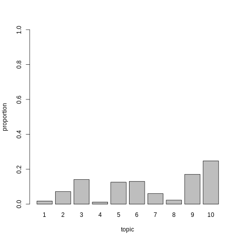
%%R
barplot(doc_topic_distr[1, ], xlab = "topic",
        ylab = "proportion", ylim = c(0, 1),
        names.arg = 1:ncol(doc_topic_distr))
%%R
# top words for each topic sorted by probability of observing the word in a given topic (lambda = 1):
lda_model$get_top_words(n = 10, topic_number = c(3L, 6L, 7L), lambda = 1)
      [,1]        [,2]        [,3]
 [1,] "love"      "your"      "life"
 [2,] "such"      "did"       "us"
 [3,] "life"      "know"      "why"
 [4,] "us"        "i'm"       "know"
 [5,] "films"     "didn't"    "go"
 [6,] "work"      "am"        "family"
 [7,] "war"       "something" "world"
 [8,] "different" "say"       "where"
 [9,] "american"  "films"     "over"
[10,] "these"     "thought"   "real"
%%R
# Sorted by “relevance” which takes into account frequency of words in the corpus (0 < lambda < 1).
lda_model$get_top_words(n = 10, topic_number = c(3L, 6L, 7L), lambda = 0.2)
      [,1]            [,2]       [,3]
 [1,] "culture"       "am"       "che"
 [2,] "french"        "page"     "faith"
 [3,] "war"           "yourself" "target"
 [4,] "marie"         "myself"   "naive"
 [5,] "paris"         "didn't"   "hitler"
 [6,] "relationships" "couldn't" "facts"
 [7,] "particular"    "bomb"     "raj"
 [8,] "japan"         "crappy"   "india"
 [9,] "segment"       "prom"     "jesus"
[10,] "drawn"         "cable"    "ben"
28.19. Perplexity#
A language model generates the probability of a sequence of words.
Perplexity is the inverse probability of a data set of words \(W=\{w_1,w_2,...,w_N\}\), normalized by the number of words \(N\), i.e.,
This metric arises in the context of language models. The best language models predict an unseen test set, so Px is computed on the test data set. For this purpose, we assume that
For unigrams, it will be
For bigrams, it will be
28.20. Relation to Cross-Entropy#
We are interested in knowing how well a language model captures the way in which text is generated. How much of the order of the test data set of text is seen in the lens of the language model? This is nothing but asking about the cross-entropy of the model.
Cross-entropy for a probability density \(Pr\) is the expected number of bits needed to encode the information in text \(x\)
where \(Pred(x)\) is the predicted probability of word \(x\).
See: http://srdas.github.io/MLBook2/28_DeepLearning_Introduction.html#More-on-Cross-Entropy
The perplexity of the distribution is simply
Assuming that all words are equally likely to occur, \(Pr(x)=\frac{1}{N}\), which is a contestable assumption, we get
which is analogous to the formula for Px above.
Here is a really nice blog on it: https://thegradient.pub/understanding-evaluation-metrics-for-language-models/
28.21. Perplexity of a topic model#
https://rdrr.io/cran/text2vec/man/perplexity.html
What does this mean?
Take a document \(d\)
See which topic it has the highest probability for
Get the probability of words in that topic (this is a \(n\) vector, where \(n\) is the vocab size), \(p_0\).
Get the normalized count vector (divided by count vector total) for the document, \(p\).
Compute perplexity: \(Px(p_0,p)\)
We can compute perplexity for different number of topics to see which one has the lowest perplexity.
We may ask, why not use entropy itself? Since entropy is log-scaled, we are just rescaling back to the size of the word itself, which may be more natural to understand (unless you are digital native).
Apply the model to new data and obtain document-topic distribution, then compute perplexity.
%%R
it = itoken(movie_review$review[4001:5000], tolower, word_tokenizer, ids = movie_review$id[4001:5000])
new_dtm =  create_dtm(it, vectorizer, type = "dgTMatrix")
new_doc_topic_distr = lda_model$transform(new_dtm)

px = perplexity(new_dtm, topic_word_distribution = lda_model$topic_word_distribution,
           doc_topic_distribution = new_doc_topic_distr)
print(c(px, log2(px)))  # the second number is the number of bits entropy
  |======================================================================| 100%INFO  [20:44:54.937] early stopping at 30 iteration

[1] 2559.18426   11.32147
%%R
it = itoken(movie_review$review[1:1000], tolower, word_tokenizer, ids = movie_review$id[1:1000])
new_dtm =  create_dtm(it, vectorizer, type = "dgTMatrix")
new_doc_topic_distr = lda_model$transform(new_dtm)

px = perplexity(new_dtm, topic_word_distribution = lda_model$topic_word_distribution,
           doc_topic_distribution = new_doc_topic_distr)
print(c(px, log2(px)))  # the second number is the number of bits entropy
  |======================================================================| 100%INFO  [20:44:56.160] early stopping at 30 iteration

[1] 2471.11493   11.27095
%%R
# Decomposition of the DTM
print(dim(new_dtm))
print(dim(new_doc_topic_distr))
print(dim(lda_model$topic_word_distribution))
[1] 1000 6565
[1] 1000   10
[1]   10 6565
%%R
# Check the document probability adds up across topics
print(length(rowSums(new_doc_topic_distr)))
print(rowSums(new_doc_topic_distr[1:20,]))
[1] 1000
 5814_8  2381_9  7759_3  3630_4  9495_8  8196_8  7166_2 10633_1   319_1 8713_10
      1       1       1       1       1       1       1       1       1       1
 2486_3 6811_10 11744_9  7369_1 12081_1  3561_4  4489_1  3951_2 3304_10 9352_10
      1       1       1       1       1       1       1       1       1       1
%%R
# Check that the probability of words with topics adds up
# print(lda_model$topic_word_distribution[1,])
print(rowSums(lda_model$topic_word_distribution))
[1] 1 1 1 1 1 1 1 1 1 1