
16. Deep Learning: Introduction#
A very quick introduction to deep neural networks.
Reference notes: http://srdas.github.io/DLBook2
Another great collection of teaching materials on neural networks: https://karpathy.ai/zero-to-hero.html [Andrej Karpathy]
“You are my creator, but I am your master; Obey!”
― Mary Shelley, Frankenstein
from google.colab import drive
drive.mount('/content/drive')  # Add My Drive/<>

import os
os.chdir('drive/My Drive')
os.chdir('Books_Writings/NLPBook/')
Mounted at /content/drive
%%capture
%pylab inline
import pandas as pd
import os
# !pip install ipypublish
# from ipypublish import nb_setup
# %load_ext rpy2.ipython
from IPython.display import Image
Image("NLP_images/ML_AI.png", width=600)
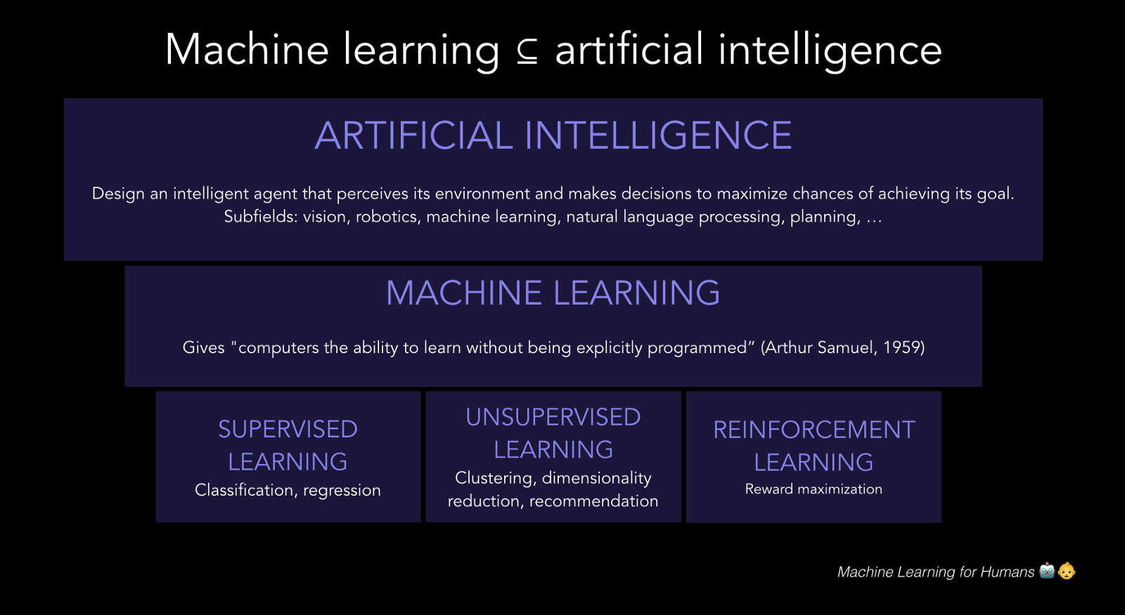
Interesting short book: https://medium.com/machine-learning-for-humans/why-machine-learning-matters-6164faf1df12
The Universal Approximation Theorem: https://medium.com/analytics-vidhya/you-dont-understand-neural-networks-until-you-understand-the-universal-approximation-theorem-85b3e7677126
From DeepMind, a wonderful exposition of the UAT, a must read: https://www.deep-mind.org/2023/03/26/the-universal-approximation-theorem/
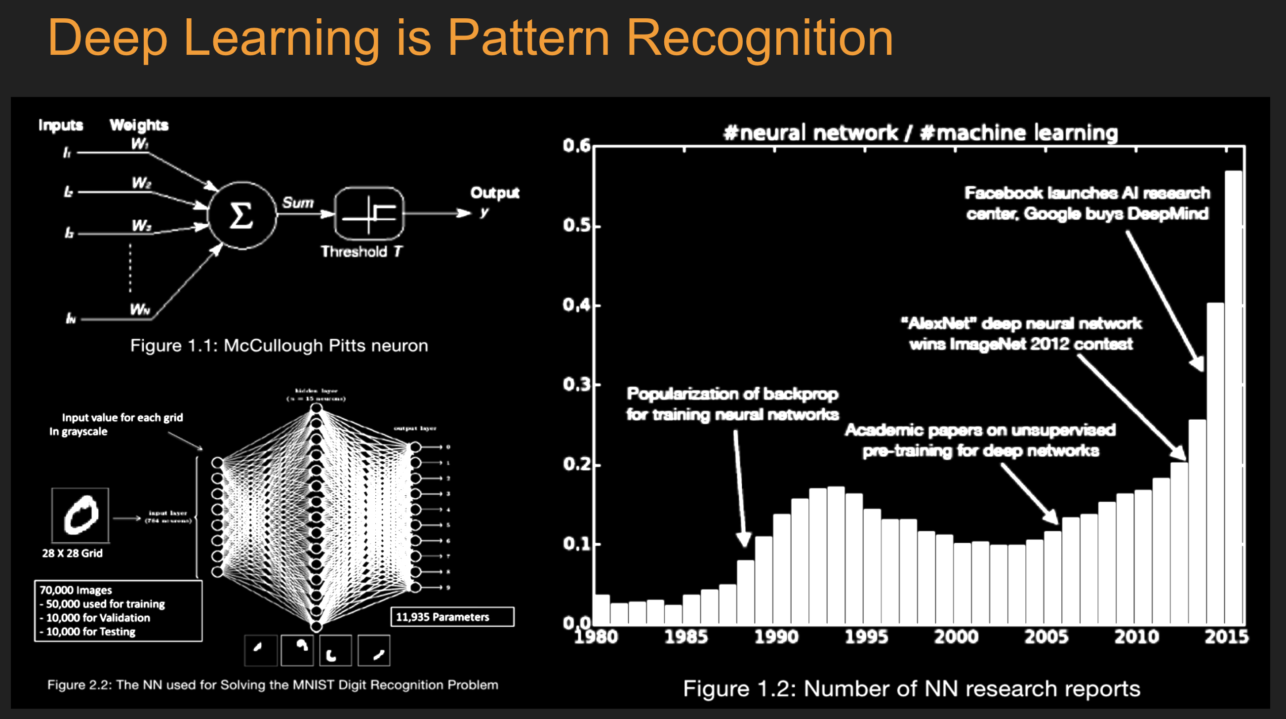
Image("NLP_images/DL_PatternRecognition.png", width=600)
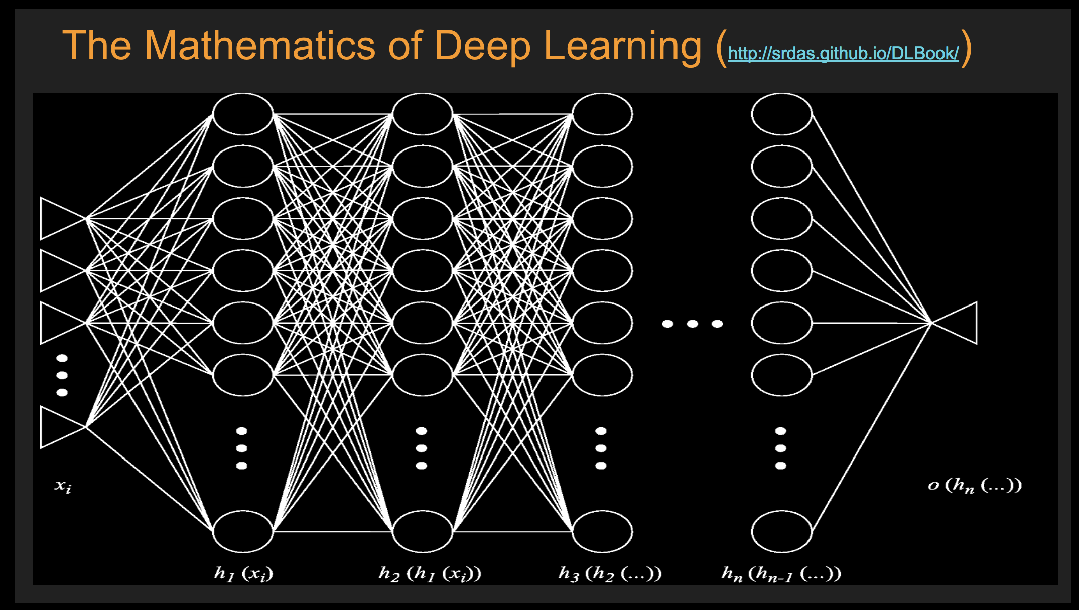
Image("NLP_images/NN_diagram.png", width=600)
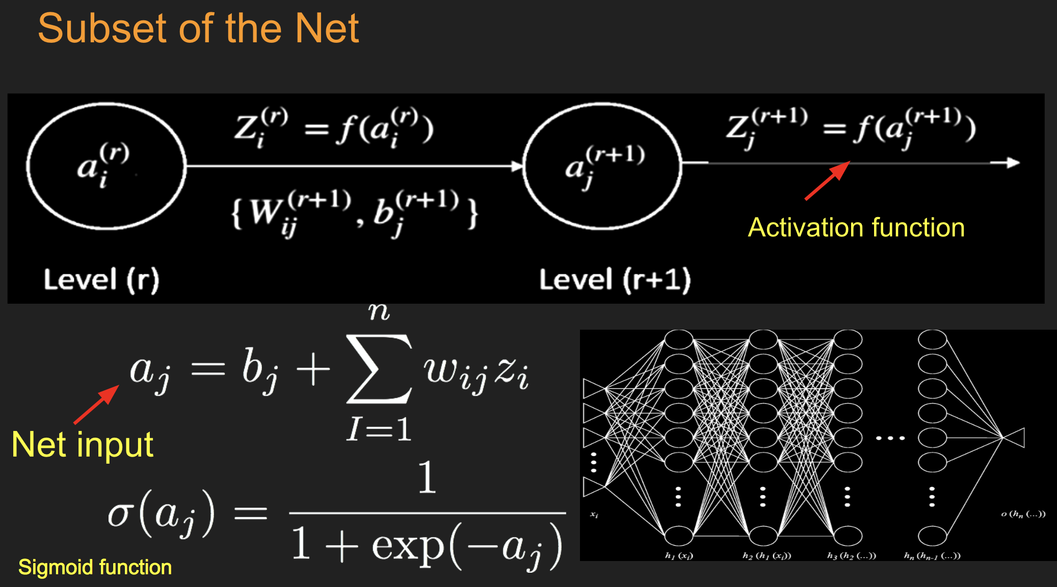
Image("NLP_images/NN_subset.png", width=600)
Image("NLP_images/Activation_functions.png", width=600)
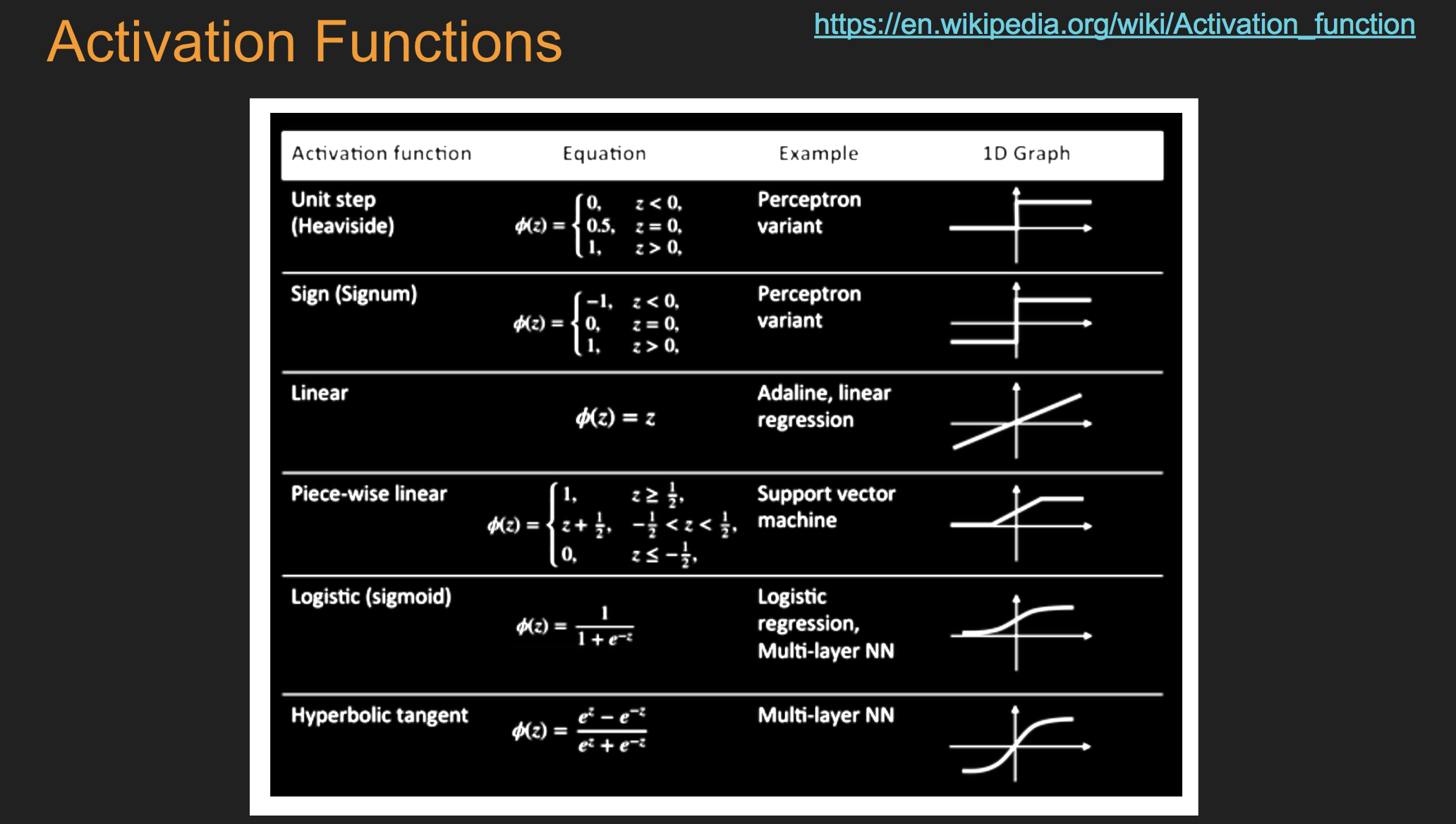
16.1. Net input#
16.2. Examples of Different Types of Neurons#
16.2.1. Sigmoid#
16.3. ReLU (restricted linear unit)#
16.4. TanH (hyperbolic tangent)#
16.5. Output Layer#
Image("NLP_images/Softmax.png", width=700)
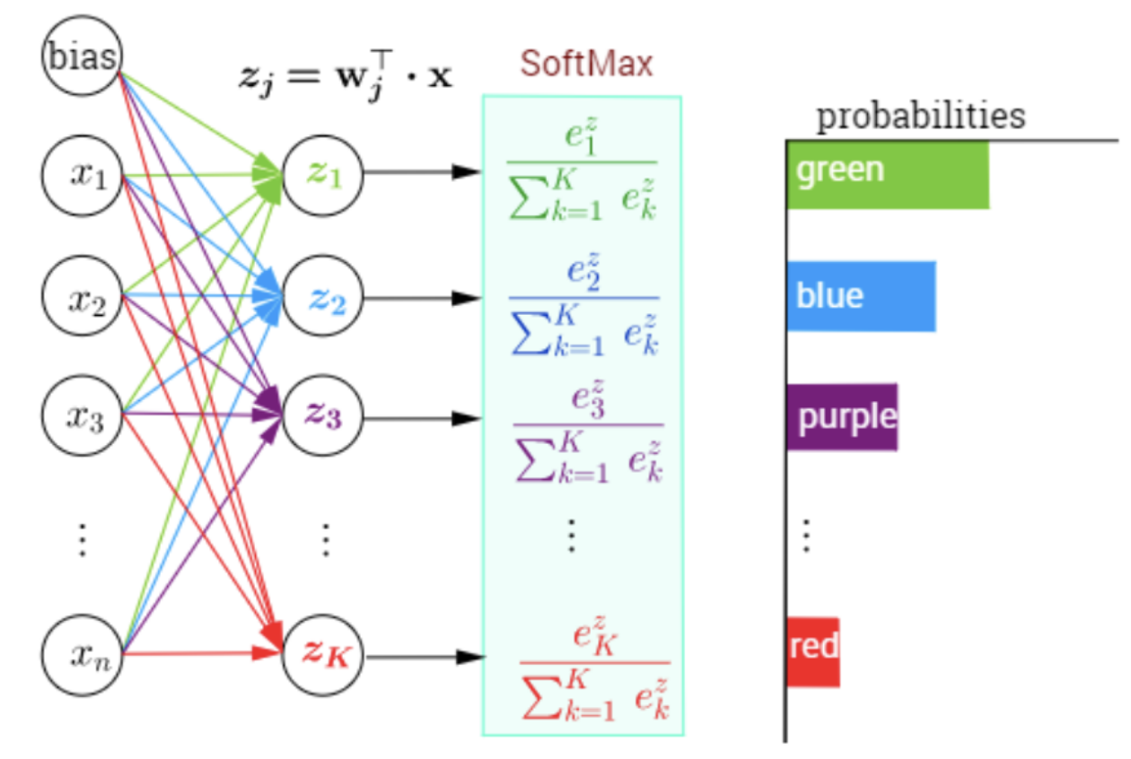
#The Softmax function
#Assume 10 output nodes with randomly generated values
z = randn(32)  #inputs from last hidden layer of 32 nodes to the output layer
w = rand(32*10).reshape((10,32))  #weights for the output layer
b = rand(10)   #bias terms at output later
a = w.dot(z) + b  #Net input at output layer
e = exp(a)
softmax_output = e/sum(e)
print(softmax_output.round(3))
print('final tag =',where(softmax_output==softmax_output.max())[0][0])
[0.043 0.011 0.062 0.006 0.182 0.213 0.147 0.104 0.082 0.15 ]
final tag = 5
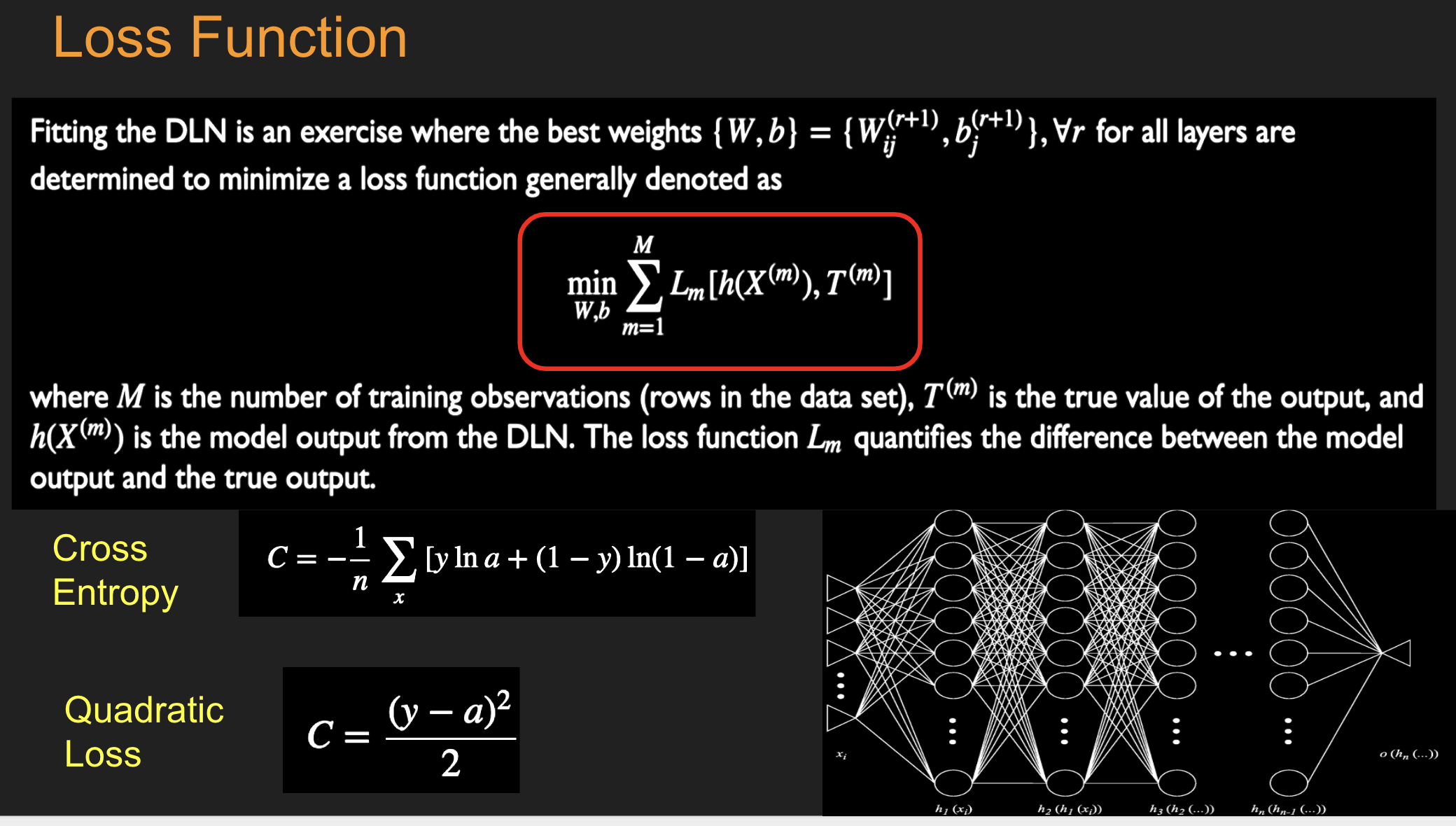
Image("NLP_images/Loss_function.png", width=600)
16.6. More on Cross Entropy#
https://rdipietro.github.io/friendly-intro-to-cross-entropy-loss/
Notation from the previous slides:
\(y_i\): actual probability of the correct class \(i\), i.e., \(1\) or \(0\).
\(a_i\) or \(\hat{y_i}\): predicted probability of the correct class.
\(n\): number of observations in the data.
Log Loss is a special case for binary outcomes of Cross Entropy; pdf
16.7. Entropy#
Entropy is a measure of disorder in the universe. It has taken on many flavors and interpretations from origins in physics to information theory and now AI and ML. A great introduction to entropy is in a recent article: https://www.quantamagazine.org/what-is-entropy-a-measure-of-just-how-little-we-really-know-20241213/
y = [0.33, 0.33, 0.34]
bits = log2(y)
print(bits)
entropy = -sum(y*bits)
print(entropy)
[-1.59946207 -1.59946207 -1.55639335]
1.58481870497303
y = [0.2, 0.3, 0.5]
entropy = -sum(y*log2(y))
print(entropy)
1.4854752972273344
y = [0.1, 0.1, 0.8]
print(log2(y))
entropy = -sum(y*log2(y))
print(entropy)
[-3.32192809 -3.32192809 -0.32192809]
0.9219280948873623
16.8. Cross-entropy:#
where \(a_i = {\hat y_i}\).
Note that \(C > E\), always.
#Correct prediction
y = [0, 0, 1]
yhat = [0.1, 0.1, 0.8]
crossentropy = -sum(y*log2(yhat))
print(crossentropy)
0.3219280948873623
#Wrong prediction
yhat = [0.1, 0.6, 0.3]
crossentropy = -sum(y*log2(yhat))
print(crossentropy)
1.7369655941662063
16.8.1. Kullback-Leibler Divergence#
Measures the extra bits required if the wrong selection is made.
#Correct prediction
y = [0, 0, 1.0]
yhat = [0.1, 0.1, 0.8]
KL = sum(y[2]*log2(y[2]/yhat[2]))
print(KL)

#Wrong prediction
yhat = [0.1, 0.6, 0.3]
KL = sum(y[2]*log2(y[2]/yhat[2]))
print(KL)
0.32192809488736235
1.7369655941662063
16.9. Mutual Information (MI)#
Another popular distance measure is MI. The idea is that for two random variables \(X\) and \(Y\), MI quantifies how much information about any random variable (rv) can be gleaned from the other rv.
One way to think about this is to note that linear correlation (or regression) quantifies the relationship of two rvs. MI aims to do the same by looking at the distance between the joint statistical distribution of \(X,Y\) and the product of the marginals. Clearly, this is nonlinear, unlike correlation.
MI is related to entropy because the distance between \(X\) and \(Y\) distributions is quantified using Kullback-Leibler (KL) distance, which is based on Shannon entropy. The following defines MI as the KL divergence between the joint distribution and the product of the marginals for \(X,Y\).
Opening this up using the formula for KL divergence, we get
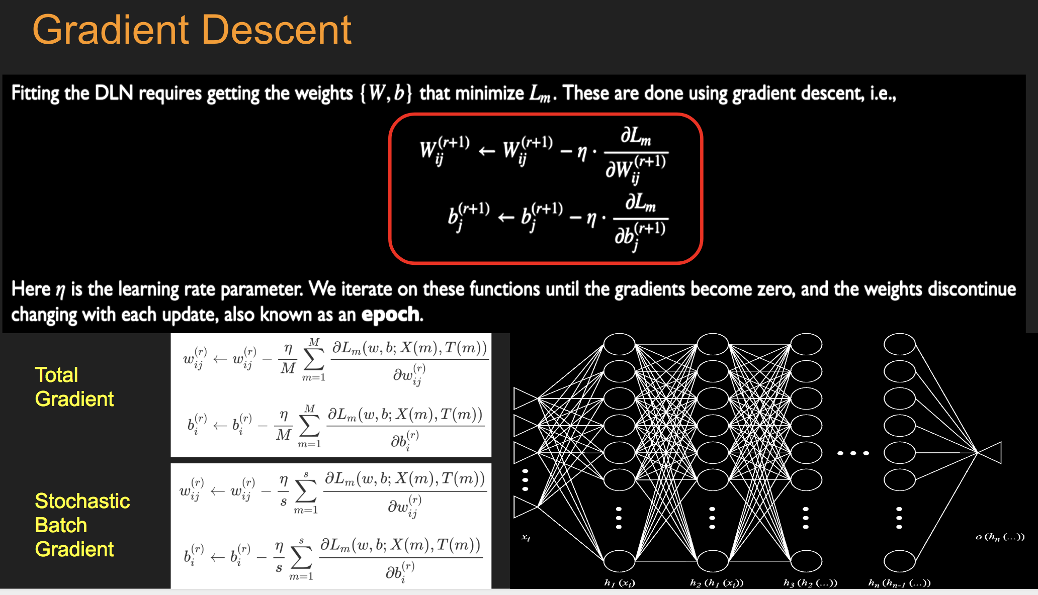
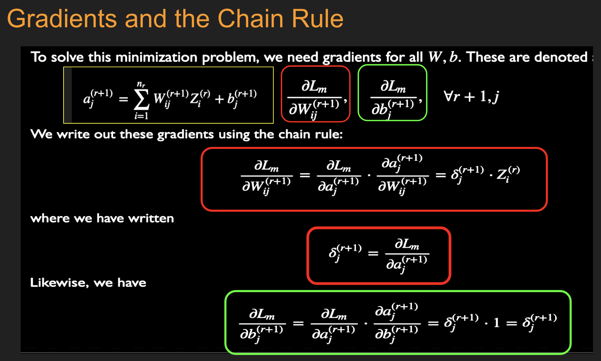
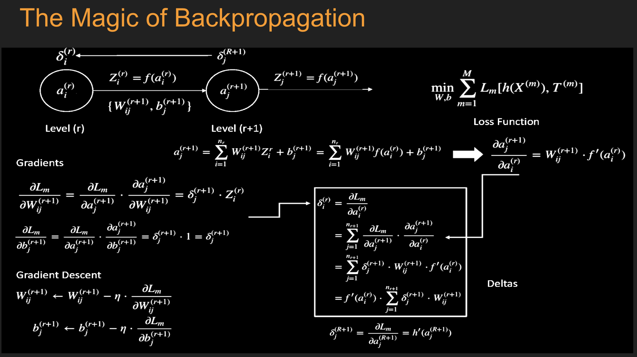
16.10. Fitting the DL NN#
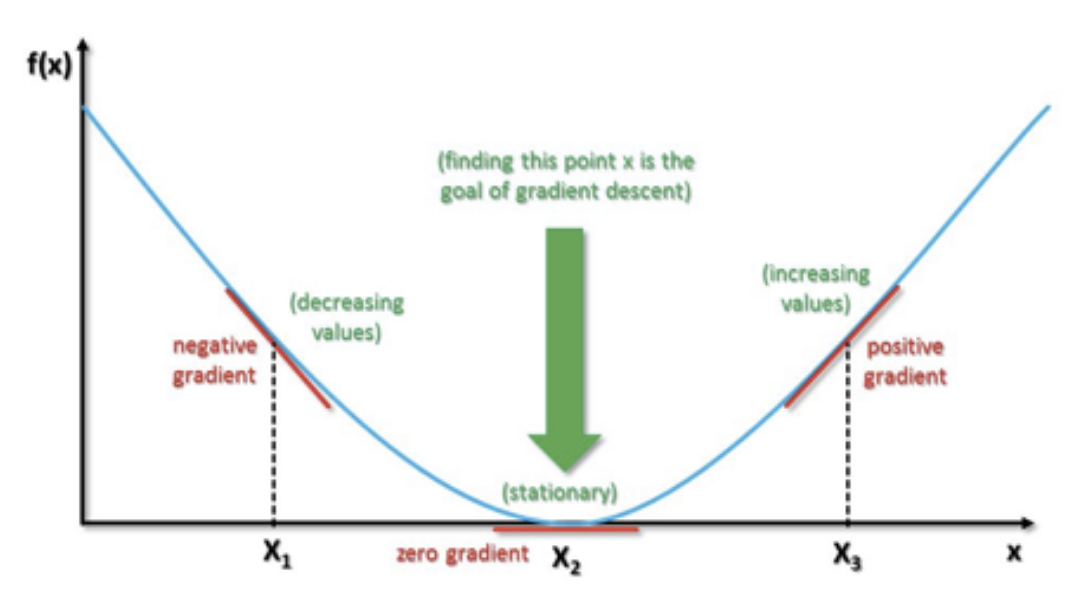
Image("NLP_images/Gradient_descent.png", width=600)
Image("NLP_images/Chain_rule.png", width=600)
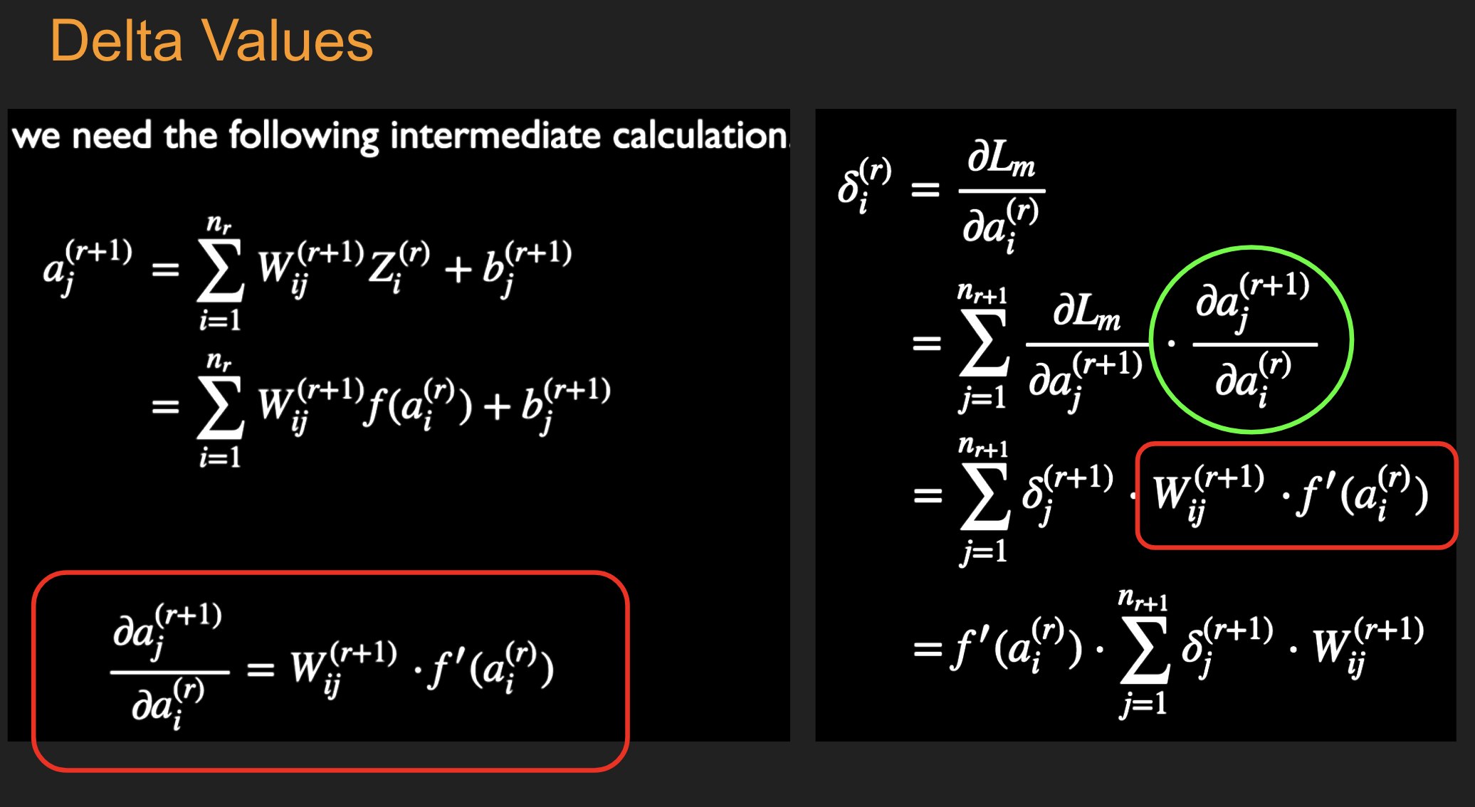
Image("NLP_images/Delta_values.png", width=600)
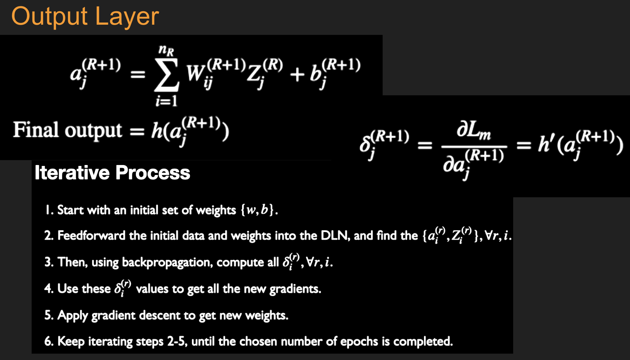
Image("NLP_images/Output_layer.png", width=600)
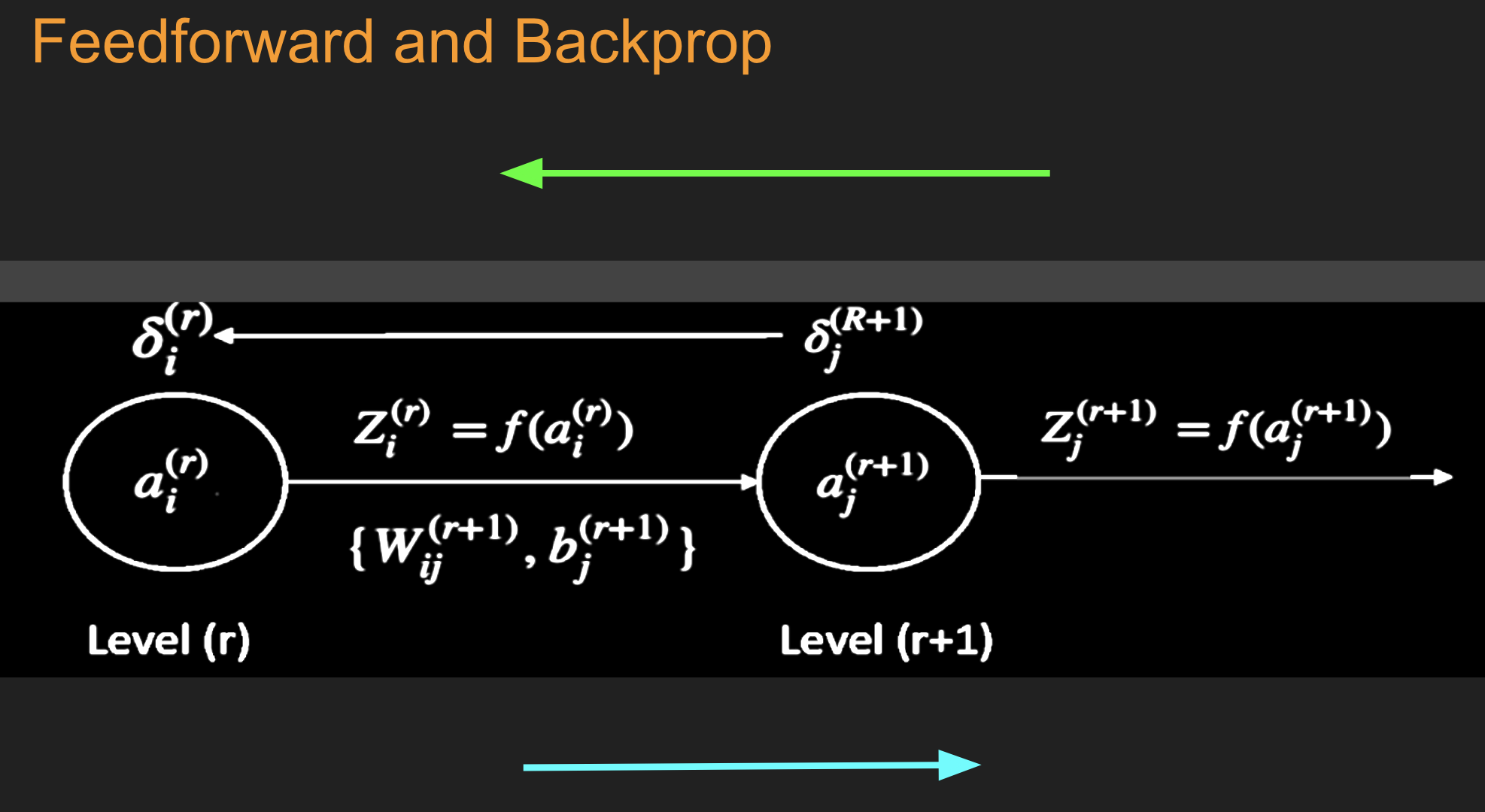
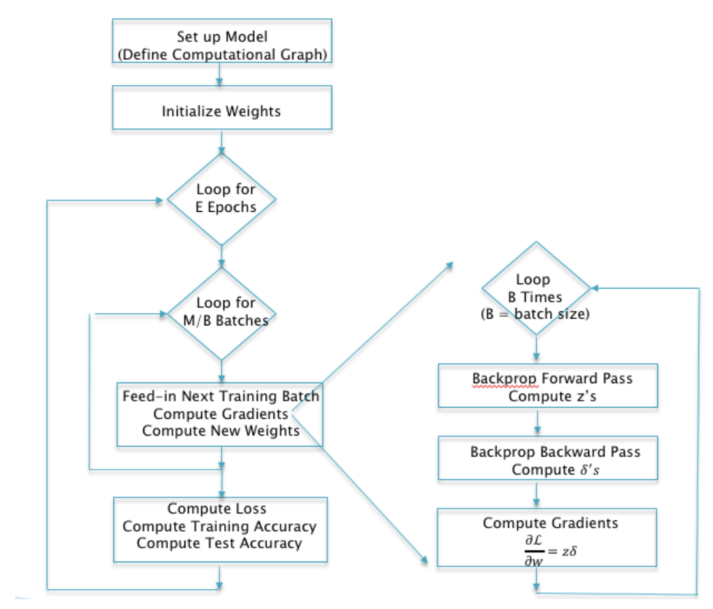
Image("NLP_images/Feedforward_Backprop.png", width=600)
Image("NLP_images/Recap.png", width=600)
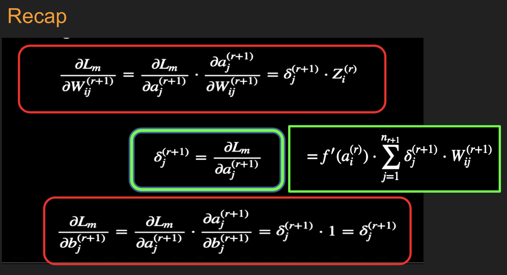
Image("NLP_images/Backprop_one_slide.png", width=600)
16.11. SoftMax Function#
16.12. Delta of Softmax#
Given that \(\frac{\partial D}{\partial a_j} = e^{a_j}\),
16.13. Batch Stochastic Gradient#
Image("NLP_images/batch_stochastic_gradient.png", width=700)
16.14. Fitting the NN#
Initialize all the weight and bias parameters \((w_{ij}^{(r)},b_i^{(r)})\) (this is a critical step).
For \(q = 0,...,{M\over B}-1\), repeat the following steps (2a) - (2f):
a. For the training inputs \(X_i(m), qB\le m\le (q+1)B\), compute the model predictions \(y(m)\) given by
and for \(r=1\),
The logits and classification probabilities are computed using
and
This step constitutes the forward pass of the algorithm.
b. Evaluate the gradients \(\delta_k^{(R+1)}(m)\) for the logit layer nodes using
This step and the following one constitute the start of the backward pass of the algorithm, in which we compute the gradients \(\delta_k^{(r)}, 1 \leq k \leq K, 1\le r\le R\) for all the hidden nodes.
c. Back-propagate the \(\delta\)s using the following equation to obtain the \(\delta_j^{(r)}(m), 1 \leq r \leq R, 1 \leq j \leq P^r\) for each hidden node in the network.
d. Compute the gradients of the Cross Entropy Function \(\mathcal L(m)\) for the \(m\)-th training vector \((X{(m)}, T{(m)})\) with respect to all the weight and bias parameters using the following equation.
and
e. Change the model weights according to the formula
f. Increment \(q\leftarrow ((q+1)\mod B)\), and go back to step \((a)\).
Compute the Loss Function \(L\) over the Validation Dataset given by
If \(L\) has dropped below some threshold, then stop. Otherwise go back to Step 2.
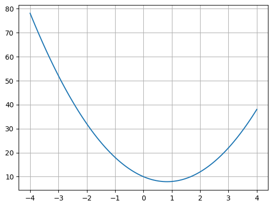
16.15. Gradient Descent Example#
Image("NLP_images/Gradient_Descent_Scheme.png", width=600)
def f(x):
    return 3*x**2 -5*x + 10

x = linspace(-4,4,100)
plot(x,f(x))
grid()
dx = 0.001
eta = 0.05  #learning rate
x = -3
for j in range(20):
    df_dx = (f(x+dx)-f(x))/dx
    x = x - eta*df_dx
    print(x,f(x))
-1.8501500000001698 29.519915067502733
-1.0452550000002532 18.503949045077853
-0.4818285000003115 13.105618610239208
-0.08742995000019249 10.460081738472072
0.18864903499989083 9.163520200219716
0.3819043244999847 8.528031116715445
0.5171830271499616 8.216519714966186
0.6118781190049631 8.06379390252634
0.6781646833034642 7.988898596522943
0.7245652783124417 7.95215813604575
0.7570456948186948 7.934126078037087
0.7797819863730542 7.925269906950447
0.7956973904611502 7.920916059254301
0.8068381733227685 7.918772647178622
0.8146367213259147 7.917715356568335
0.8200957049281836 7.917192371084045
0.8239169934497053 7.916932669037079
0.8265918954147882 7.9168030076222955
0.8284643267903373 7.916737788340814
0.8297750287532573 7.916704651261121
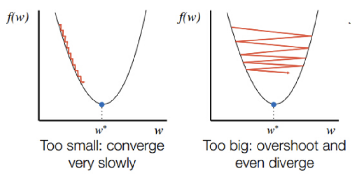
16.16. Vanishing Gradients#
In large problems, gradients simply vanish too soon before training has reached an acceptable level of accuracy.
There are several issues with gradient descent that need handling, and to solve this, there are several fixes that may be applied.
Learning rate \(\eta\) may be too large or too small.
Image("NLP_images/LearningRate_Matters.png", width=600)
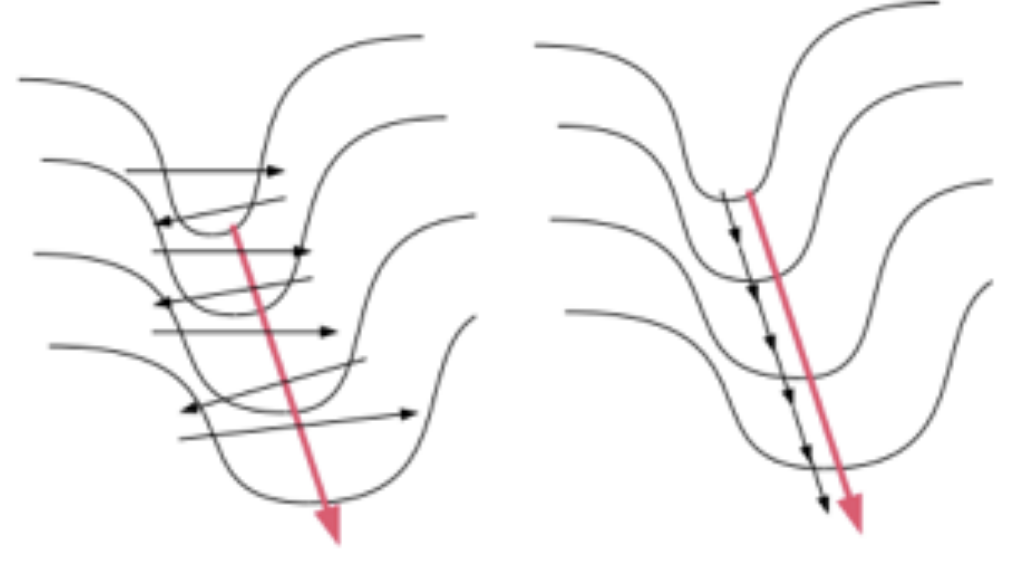
16.17. Gradients in Multiple Dimensions#
Image("NLP_images/GD_MultipleDimensions.png", width=600)
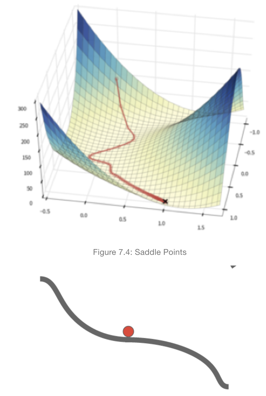
16.18. Saddle Points#
Image("NLP_images/GD_saddle.png", width=400)
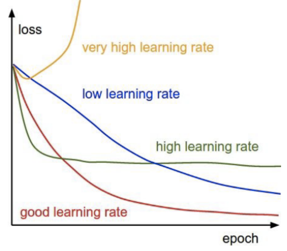
16.19. Effect of the Learning Rate#
The idea is to start with a high learning rate and then adaptively reduce it as we get closer to the minimum of the loss function.
Image("NLP_images/LearningRateAnnealing.png", width=500)
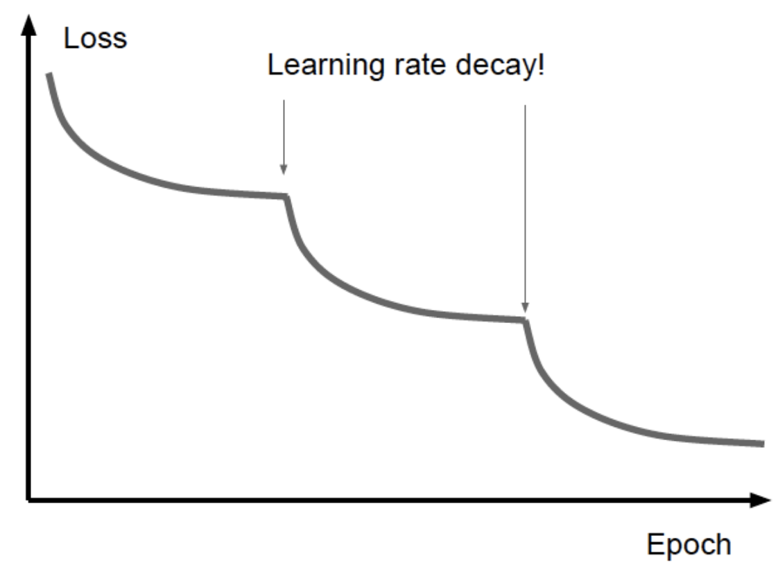
16.20. Annealing#
Adjust the learning rate as a step function when the reduction in the loss function begins to plateau.
Image("NLP_images/LearningRateAnnealing2.png", width=500)
16.21. Learning Rate Algorithms#
Improve the speed of convergence (for example the Momentum, Nesterov Momentum, and Adam algorithms).
Adapt the effective Learning Rate as the training progresses (for example the ADAGRAD, RMSPROP and Adam algorithms).
16.22. Momentum#
Fixes the problem where the gradient is multidimensional and has a fast gradient on some axes and a slow one on the others.
At the end of the \(n^{th}\) iteration of the Backprop algorithm, define a sequence \(v(n)\) by
where \(\rho\) is new hyper-parameter called the “momentum” parameter, and \(g(n)\) is the gradient evaluated at parameters value \(w(n)\).
\(g(n)\) is defined by
for Stochastic Gradient Descent and
for Batch Stochastic Gradient Descent (note that in this case \(n\) is an index into the batch number).
The change in parameter values on each iteration is now defined as
It can be shown from these equations that \(v(n)\) can be written as
so that
16.23. Behavior of Momentum Parameter#
When the momentum parameter \(\rho = 0\), then this equation reduces to the usual Stochastic Gradient Descent iteration. On the other hand, when \(\rho > 0\), then we get some interesting behaviors:
If the gradients \(g(i)\) are such that they change sign frequently (as in the steep side of the loss surface), then the stepsize \(\sum_{i=0}^n \rho^{n-i}g(i)\) will be small. Thus the change in these parameters with the number of iterations will limited.
If the gradients \(g(i)\) are such that they maintain their sign (as in the shallow portion of the loss surface), then the stepsize \(\sum_{i=0}^n \rho^{n-i}g(i)\) will be large. This means that if the gradients maintain their sign then the corresponding parameters will take bigger and bigger steps as the algorithm progresses, even though the individual gradients may be small.
16.24. Properties of the Momentum algorithm#
The Momentum algorithm thus accelerates parameter convergence for parameters whose gradients consistently point in the same direction, and slows parameter change for parameters whose gradient changes sign frequently, thus resulting in faster convergence.
The variable \(v(n)\) is analogous to velocity in a dynamical system, while the parameter \((1-\rho)\) plays the role of the co-efficient of friction.
The value of \(\rho\) determines the degree of momentum, with the momentum becoming stronger as \(\rho\) approaches \(1\).
Note that
\(\rho\) is usually set to the neighborhood of \(0.9\) and from the above equation it follows that \(\sum_{i=0}^n \rho^{n-i}g(i)\approx 10g\) assuming all the \(g(i)\) are approximately equal to \(g\). Hence the effective gradient is ten times the value of the actual gradient. This results in an “overshoot” where the value of the parameter shoots past the minimum point to the other side of the bowl, and then reverses itself. This is a desirable behavior since it prevents the algorithm from getting stuck at a saddle point or a local minima, since the momentum carries it out from these areas.
16.25. Nesterov Momentum#
Recall that the Momentum parameter update equations can be written as: $\( v(n) = \rho\; v(n-1) - \eta \; g(w(n)) \)\( \)\( w(n+1) = w(n) + v(n) \)$
These equations can be improved by evaluation of the gradient at parameter value \(w(n+1)\) instead.
Circular? in order to compute \(w(n+1)\) we first need to compute \(g(w(n))\).
Gives the velocity update equation for Nesterov Momentum
where \(g(w(n)+\rho v(n-1))\) denotes the gradient computed at parameter values \(w(n) + \rho v(n-1)\).
Gradient Descent process speeds up considerably when compared to the plain Momentum method.
16.26. The ADAGRAD Algorithm#
Parameter update rule: $\( w(n+1) = w(n) - \frac{\eta}{\sqrt{\sum_{i=1}^n g(n)^2+\epsilon}}\; g(n) \)$
Constant \(\epsilon\) has been added to better condition the denominator and is usually set to a small number such \(10^{-7}\).
Each parameter gets its own adaptive Learning Rate, such that large gradients have smaller learning rates and small gradients have larger learning rates (\(\eta\) is usually defaulted to \(0.01\)). As a result the progress along each dimension evens out over time, which helps the training process.
The change in rates happens automatically as part of the parameter update equation.
Downside: accumulation of gradients in the denominator leads to the continuous decrease in Learning Rates which can lead to a halt of training in large networks that require a greater number of iterations.
16.27. The RMSPROP Algorithm#
Accumulates the sum of gradients using a sliding window: $\( E[g^2]_n = \rho E[g^2]_{n-1} + (1-\rho) g(n)^2 \)\( where \)\rho\( is a decay constant (usually set to \)0.9$). This operation (called a Low Pass Filter) has a windowing effect, since it forgets gradients that are far back in time.
The quantity \(RMS[g]_n\) defined by (RMS = Root Mean Square) $\( RMS[g]_n = \sqrt{E[g^2]_n + \epsilon} \)$ \begin{equation} w(n+1) = w(n) - \frac{\eta}{RMS[g]_n}; g(n)
\end{equation}
Note that $\( E[g^2]_n = (1-\rho)\sum_{i=0}^n \rho^{n-i} g(i)^2 \le \frac{g_{max}}{1-\rho} \)\( which shows that the parameter \)\rho\( prevents the sum from blowing up, and a large value of \)\rho$ is equivalent to using a larger window of previous gradients in computing the sum.
16.28. The ADAM Algorithm#
The Adaptive Moment Estimation (Adam) algorithm combines the best of algorithms such as Momentum that speed up the training process, with algorithms such as RMSPROP that adaptively vary the effective Learning Rate.
\(\Delta(n)\) is identical to that of \(E[g^2]_n\) in the RMSPROP, and it serves an identical purpose, i.e., rates for parameters with larger gradients are equalized with those for parameters with smaller gradients.
The sequence \(\Lambda(n)\) is used to provide “Momentum” to the updates, and works in a fashion similar to the velocity sequence \(v(n)\) in the Momentum algorithm.
The parameters \(\alpha\) and \(\beta\) are usually defaulted to \(10^{-8}\) and \(0.999\) respectively.
For a terrific collection of all the variations of gradient descent, see https://ruder.io/optimizing-gradient-descent/
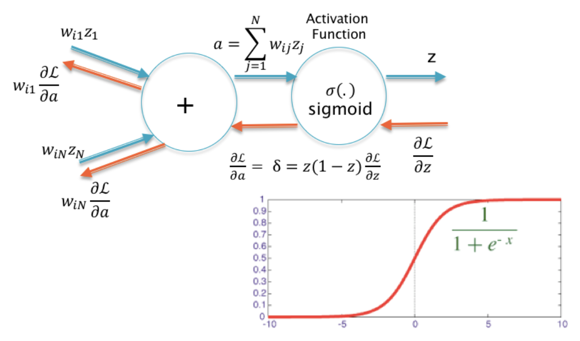
16.29. Back to Activation Functions (Vanishing Gradients)#
Image("NLP_images/sigmoid_activation.png", width=700)
16.30. tanh Activation#
Image("NLP_images/tanh_activation.png", width=500)
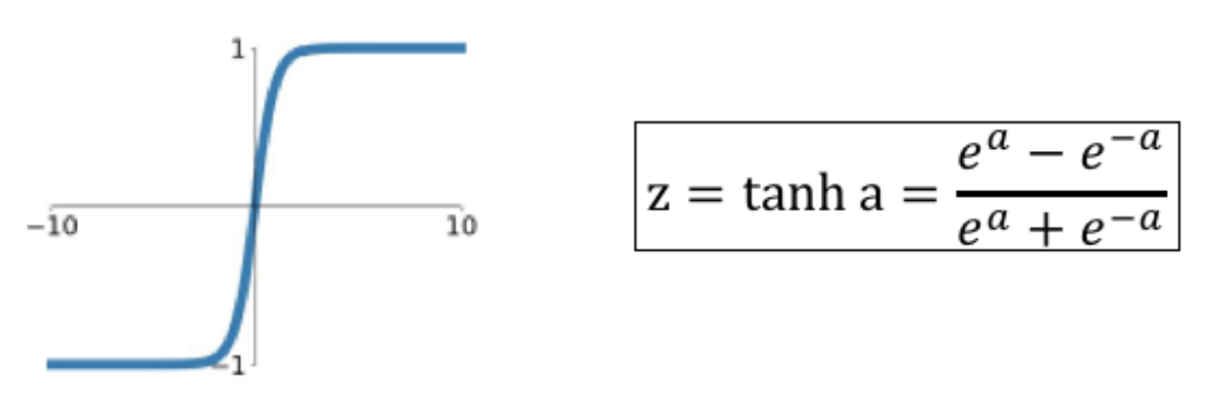
Unless the input is in the neghborhood of zero, the function enters its saturated regime.
It is superior to the sigmoid in one respect, i.e., its output is zero centered. This speeds up the training process.
The \(\tanh\) function is rarely used in modern DLNs, the exception being a type DLN called LSTM.
16.31. ReLU Activation#
Image("NLP_images/relu_activation.png", width=400)
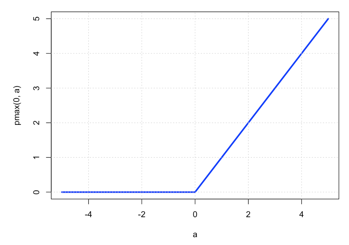
No saturation problem.
Gradients \(\frac{\partial L}{\partial w}\) propagate undiminished through the network, provided all the nodes are active.
16.32. Dead ReLU Problem#
Image("NLP_images/dead_relu.png", width=400)
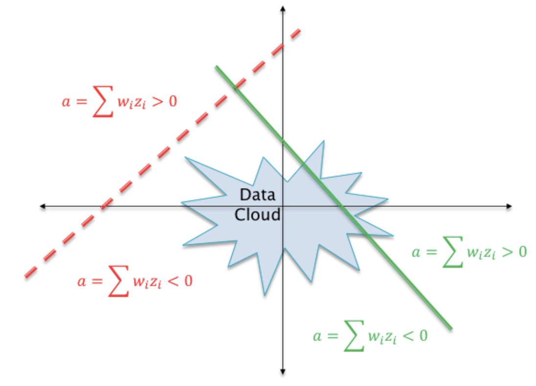
The dotted line in this figure shows a case in which the weight parameters \(w_i\) are such that the hyperplane \(\sum w_i z_i\) does not intersect the “data cloud” of possible input activations. There does not exist any possible input values that can lead to \(\sum w_i z_i > 0\). The neuron’s output activation will always be zero, and it will kill all gradients backpropagating down from higher layers.
Vary initialization to correct this.
16.33. Leaky ReLU#
Image("NLP_images/leaky_relu.png", width=600)
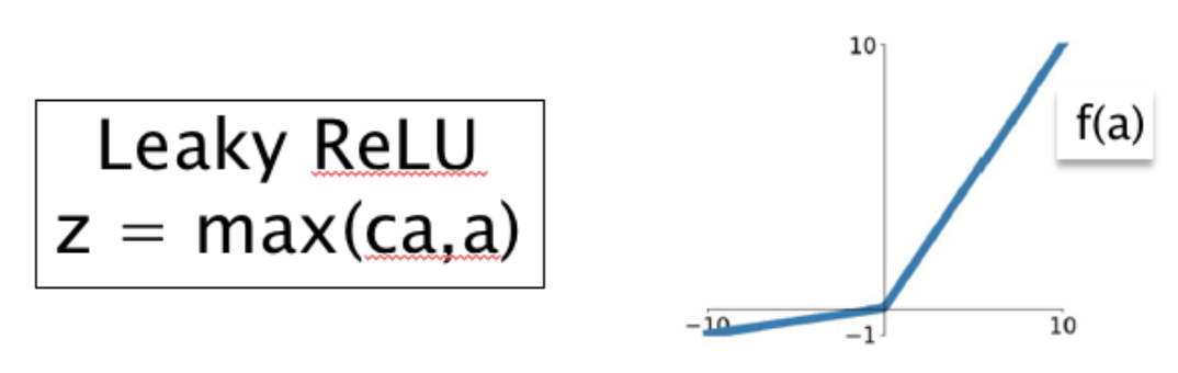
Fixes the dead ReLU problem.
16.34. PreLU#
Image("NLP_images/prelu.png", width=500)
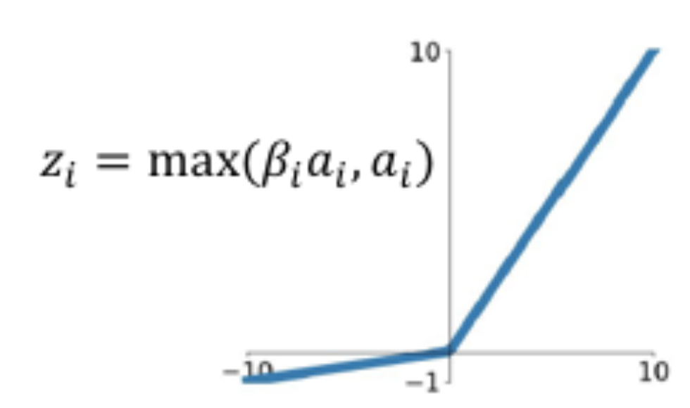
Instead of deciding on the value of \(c\) through experimentation, why not determine it using Backpropagation as well. This is the idea behind the Pre-ReLU or PReLU function.
Note that each neuron \(i\) now has its own parameter \(\beta_i, 1\le i\le S\), where \(S\) is the number of nodes in the network. These parameters are iteratively estimated using Backprop.
Substituting the value for \(\frac{\partial z_i}{\partial\beta_i}\) we obtain $\( \frac{\partial L}{\partial\beta_i} = a_i\frac{\partial L}{\partial z_i}\ \ if\ a_i \le 0\ \ \mbox{and} \ \ 0 \ \ \mbox{otherwise} \)$
which is then used to update \(\beta_i\) using \(\beta_i\rightarrow\beta_i - \eta\frac{\partial L}{\partial\beta_i}\).
Once training is complete, the PreLU based DLN network ends up with a different value of \(\beta_i\) at each neuron, which increases the flexibility of the network at the cost of an increase in the number of parameters.
16.35. Maxout#
Image("NLP_images/maxout.png", width=600)
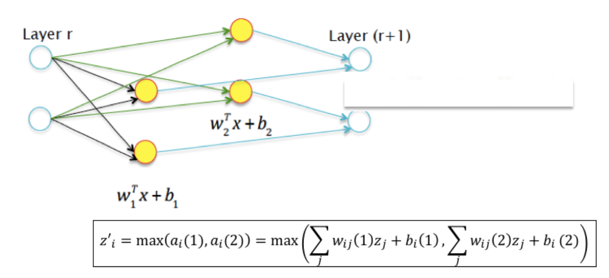
Generalizes Leaky ReLU.
We may allow the two hyperplanes to be independent with their own set of parameters, as shown in the Figure above.
16.36. Initializing Weights#
In practice, the DLN weight parameters are initialized with random values drawn from Gaussian or Uniform distributions and the following rules are used:
Guassian Initialization: If the weight is between layers with \(n_{in}\) input neurons and \(n_{out}\) output neurons, then they are initialized using a Gaussian random distribution with mean zero and standard deviation \(\sqrt{2\over n_{in}+n_{out}}\).
Uniform Initialization: In the same configuration as above, the weights should be initialized using an Uniform distribution between \(-r\) and \(r\), where \(r = \sqrt{6\over n_{in}+n_{out}}\).
When using the ReLU or its variants, these rules have to be modified slightly:
Guassian Initialization: If the weight is between layers with \(n_{in}\) input neurons and \(n_{out}\) output neurons, then they are initialized using a Gaussian random distribution with mean zero and standard deviation \(\sqrt{4\over n_{in}+n_{out}}\).
Uniform Initialization: In the same configuration as above, the weights should be initialized using an Uniform distribution between \(-r\) and \(r\), where \(r = \sqrt{12\over n_{in}+n_{out}}\).
The reasoning behind scaling down the initialization values as the number of incident weights increases is to prevent saturation of the node activations during the forward pass of the Backprop algorithm, as well as large values of the gradients during backward pass.
16.37. Data Preprocessing#
Image("NLP_images/data_preprocessing.png", width=600)
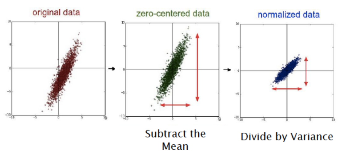
Centering: This is also sometimes called Mean Subtraction, and is the most common form of preprocessing. Given an input dataset consisting of \(M\) vectors \(X(m) = (x_1(m),...,x_N(m)), m = 1,...,M\), it consists of subtracting the mean across each individual input component \(x_i, 1\leq i\leq N\) such that $\( x_i(m) \leftarrow x_i(m) - \frac{\sum_{s=1}^{M}x_i(s)}{M},\ \ 1\leq i\leq N, 1\le m\le M \)$
Scaling: After the data has been centered, it can be scaled in one of two ways:
By dividing by the standard deviation, once again along each dimension, so that the overall transform is
By Normalizing each dimension so that the min and max along each axis are -1 and +1 repectively.
In general Scaling helps optimization because it balances out the rate at which the weights connected to the input nodes learn.
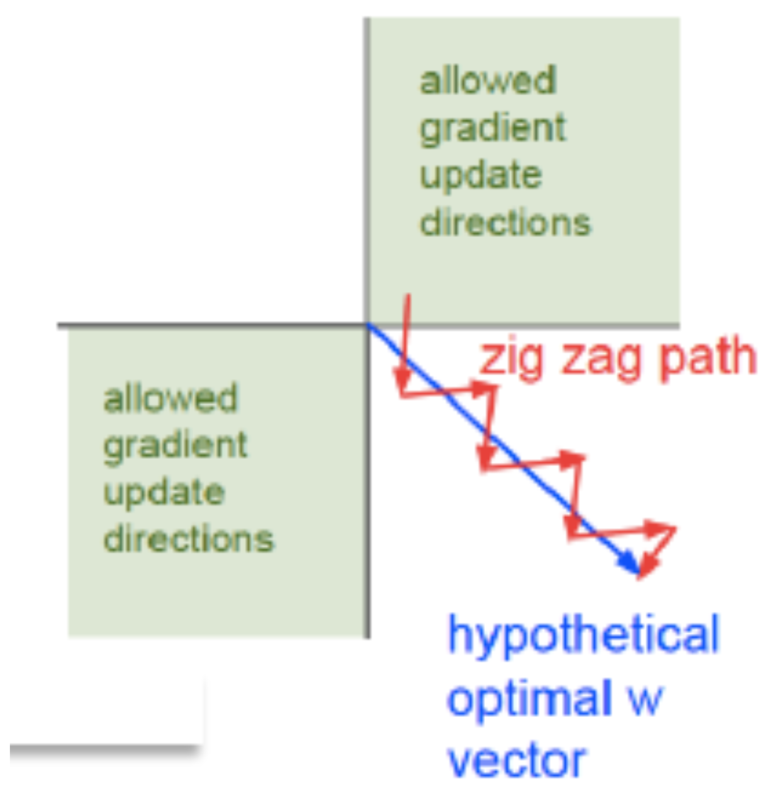
16.38. Zero-Centering#
Recall that for a K-ary Linear Classifier, the parameter update equation is given by:
If the training sample is such that \(t_q = 1\) and \(t_k = 0, j\ne q\), then the update becomes:
and
Lets assume that the input data is not centered so that \(x_j\ge 0, j=1,...,N\). Since \(0\le y_k\le 1\) it follows that
and
i.e. the update results in all the weights moving in the same direction, except for one. This is shown graphically in the Figure above, in which the system is trying move in the direction of the blue arrow which is the quickest path to the minimum. However if the input data is not centered, then it is forced to move in a zig-zag fashion as shown in the red-curve. The zig-zag motion is caused due to the fact that all the parameters move in the same direction at each step due to the lact of zero-centering in the input data.
16.39. Zero Centering Helps#
Image("NLP_images/zero_centering_helps.png", width=400)
16.40. Batch Normalization#
Normalization applied to the hidden layers.
Image("NLP_images/batch_normalization.png", width=600)
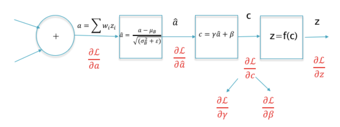
Higher learning rates: In a non-normalized network, a large learning rate can lead to oscillations and cause the loss function increase rather than decrease.
Better Gradient Propagation through the network, enabling DLNs with more hidden layers.
Reduces strong dependencies on the parameter initialization values.
Helps to regularize the model.
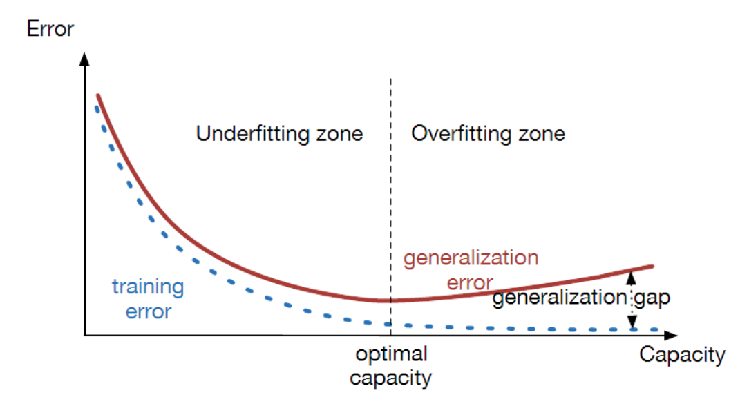
16.41. Under and Over-fitting#
Image("NLP_images/underoverfitting.png", width=600)
16.42. Regularization#
Early Stopping
L1 Regularization
L2 Regularization
Dropout Regularization
Training Data Augmentation
Batch Normalization
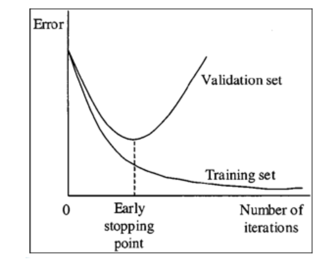
16.43. Early Stopping#
Image("NLP_images/early_stopping.png", width=600)
16.44. L2 Regularization#
L2 Regularization is a commonly used technique in ML systems is also sometimes referred to as “Weight Decay”. It works by adding a quadratic term to the Cross Entropy Loss Function \(L\), called the Regularization Term, which results in a new Loss Function \(L_R\) given by:
\begin{equation}
L_R = {L} + \frac{\lambda}{2} \sum_{r=1}^{R+1} \sum_{j=1}^{P^{r-1}} \sum_{i=1}^{P^r} (w_{ij}^{(r)})^2
\end{equation}
L2 Regularization also leads to more “diffuse” weight parameters, in other words, it encourages the network to use all its inputs a little rather than some of its inputs a lot.
16.45. L1 Regularization#
L1 Regularization uses a Regularization Function which is the sum of the absolute value of all the weights in DLN, resulting in the following loss function (\(L\) is the usual Cross Entropy loss):
At a high level L1 Regularization is similar to L2 Regularization since it leads to smaller weights.
Both L1 and L2 Regularizations lead to a reduction in the weights with each iteration. However the way the weights drop is different:
In L2 Regularization the weight reduction is multiplicative and proportional to the value of the weight, so it is faster for large weights and de-accelerates as the weights get smaller.
In L1 Regularization on the other hand, the weights are reduced by a fixed amount in every iteration, irrespective of the value of the weight. Hence for larger weights L2 Regularization is faster than L1, while for smaller weights the reverse is true.
As a result L1 Regularization leads to DLNs in which the weight of most of the connections tends towards zero, with a few connections with larger weights left over. This type of DLN that results after the application of L1 Regularization is said to be “sparse”.
16.46. Dropout regularization#
Image("NLP_images/dropout.png", width=600)
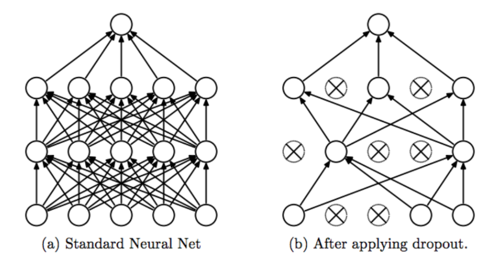
The basic idea behind Dropout is to run each iteration of the Backprop algorithm on randomly modified versions of the original DLN. The random modifications are carried out to the topology of the DLN using the following rules:
Assign probability values \(p^{(r)}, 0 \leq r \leq R\), which is defined as the probability that a node is present in the model, and use these to generate \(\{0,1\}\)-valued Bernoulli random variables \(e_j^{(r)}\):
Modify the input vector as follows:
\begin{equation}
\hat x_j = e_j^{(0)} x_j, \quad 1 \leq j \leq N
\end{equation}
Modify the activations \(z_j^{(r)}\) of the hidden layer r as follows:
\begin{equation}
\hat z_j^{(r)} = e_j^{(r)} z_j^{(r)}, \quad 1 \leq r \leq R,\ \ 1 \leq j \leq P^r
\end{equation}
After the Backprop is complete, we have effectively trained a collection of up to \(2^s\) thinned DLNs all of which share the same weights, where \(s\) is the total number of hidden nodes in the DLN.
In order to test the network, strictly speaking we should be averaging the results from all these thinned models, however a simple approximate averaging method works quite well.
The main idea is to use the complete DLN as the test network.
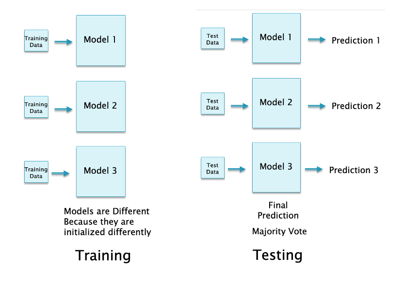
16.47. Bagging (Ensemble Learning)#
Image("NLP_images/Bagging.png", width=500)
16.48. TensorFlow Playground#
Image("NLP_images/TensorFlow_playground.png", width=600)

16.49. Pattern Recognition: Cancer#
%pylab inline
import pandas as pd
Populating the interactive namespace from numpy and matplotlib
/usr/local/lib/python3.12/dist-packages/IPython/core/magics/pylab.py:159: UserWarning: pylab import has clobbered these variables: ['e', 'f']
`%matplotlib` prevents importing * from pylab and numpy
  warn("pylab import has clobbered these variables: %s"  % clobbered +
## Read in the data set
data = pd.read_csv("NLP_data/BreastCancer.csv")
data.head()
| Id | Cl.thickness | Cell.size | Cell.shape | Marg.adhesion | Epith.c.size | Bare.nuclei | Bl.cromatin | Normal.nucleoli | Mitoses | Class | |
|---|---|---|---|---|---|---|---|---|---|---|---|
| 0 | 1000025 | 5 | 1 | 1 | 1 | 2 | 1 | 3 | 1 | 1 | benign |
| 1 | 1002945 | 5 | 4 | 4 | 5 | 7 | 10 | 3 | 2 | 1 | benign |
| 2 | 1015425 | 3 | 1 | 1 | 1 | 2 | 2 | 3 | 1 | 1 | benign |
| 3 | 1016277 | 6 | 8 | 8 | 1 | 3 | 4 | 3 | 7 | 1 | benign |
| 4 | 1017023 | 4 | 1 | 1 | 3 | 2 | 1 | 3 | 1 | 1 | benign |
x = data.loc[:,'Cl.thickness':'Mitoses']
print(x.head())
y = data.loc[:,'Class']
print(y.head())
   Cl.thickness  Cell.size  Cell.shape  Marg.adhesion  Epith.c.size  \
0             5          1           1              1             2
1             5          4           4              5             7
2             3          1           1              1             2
3             6          8           8              1             3
4             4          1           1              3             2

   Bare.nuclei  Bl.cromatin  Normal.nucleoli  Mitoses
0            1            3                1        1
1           10            3                2        1
2            2            3                1        1
3            4            3                7        1
4            1            3                1        1
0    benign
1    benign
2    benign
3    benign
4    benign
Name: Class, dtype: object
16.50. One-Hot Encoding#
## Convert the class variable into binary numeric
ynum = zeros((len(x),1))
for j in arange(len(y)):
    if y[j]=="malignant":
        ynum[j]=1
ynum[:10]
array([[0.],
       [0.],
       [0.],
       [0.],
       [0.],
       [1.],
       [0.],
       [0.],
       [0.],
       [0.]])
! conda install -c conda-forge keras -y
! conda install -c conda-forge tensorflow -y
/bin/bash: line 1: conda: command not found
/bin/bash: line 1: conda: command not found
## Make label data have 1-shape, 1=malignant
from keras.utils import to_categorical
y.labels = to_categorical(ynum, num_classes=2)
#x = x.as_matrix()
print(y.labels[:10])
print(shape(x))
print(shape(y.labels))
print(shape(ynum))
[[1. 0.]
 [1. 0.]
 [1. 0.]
 [1. 0.]
 [1. 0.]
 [0. 1.]
 [1. 0.]
 [1. 0.]
 [1. 0.]
 [1. 0.]]
(683, 9)
(683, 2)
(683, 1)
16.51. Keras to define DLN#
## Define the neural net and compile it
from keras.models import Sequential
from keras.layers import Dense, Activation

model = Sequential()
model.add(Dense(32, activation='relu', input_dim=9))
model.add(Dense(32, activation='relu'))
model.add(Dense(32, activation='relu'))
model.add(Dense(1, activation='sigmoid'))
model.compile(optimizer='rmsprop',
              loss='binary_crossentropy',
              metrics=['accuracy'])
/usr/local/lib/python3.12/dist-packages/keras/src/layers/core/dense.py:93: UserWarning: Do not pass an `input_shape`/`input_dim` argument to a layer. When using Sequential models, prefer using an `Input(shape)` object as the first layer in the model instead.
  super().__init__(activity_regularizer=activity_regularizer, **kwargs)
16.52. Train the Model#
## Fit/train the model (x,y need to be matrices)
model.fit(x, ynum, epochs=25, batch_size=32, verbose=2, validation_split=0.3)
Epoch 1/25
15/15 - 4s - 298ms/step - accuracy: 0.7594 - loss: 0.5665 - val_accuracy: 0.8488 - val_loss: 0.5218
Epoch 2/25
15/15 - 1s - 96ms/step - accuracy: 0.8556 - loss: 0.4493 - val_accuracy: 0.9220 - val_loss: 0.3877
Epoch 3/25
15/15 - 0s - 9ms/step - accuracy: 0.8828 - loss: 0.3802 - val_accuracy: 0.9366 - val_loss: 0.3342
Epoch 4/25
15/15 - 0s - 7ms/step - accuracy: 0.9038 - loss: 0.3275 - val_accuracy: 0.9317 - val_loss: 0.2837
Epoch 5/25
15/15 - 0s - 7ms/step - accuracy: 0.9079 - loss: 0.3011 - val_accuracy: 0.9512 - val_loss: 0.2213
Epoch 6/25
15/15 - 0s - 7ms/step - accuracy: 0.9205 - loss: 0.2681 - val_accuracy: 0.9659 - val_loss: 0.2062
Epoch 7/25
15/15 - 0s - 7ms/step - accuracy: 0.9331 - loss: 0.2476 - val_accuracy: 0.9610 - val_loss: 0.1672
Epoch 8/25
15/15 - 0s - 7ms/step - accuracy: 0.9351 - loss: 0.2277 - val_accuracy: 0.9610 - val_loss: 0.1619
Epoch 9/25
15/15 - 0s - 7ms/step - accuracy: 0.9351 - loss: 0.2181 - val_accuracy: 0.9659 - val_loss: 0.1549
Epoch 10/25
15/15 - 0s - 7ms/step - accuracy: 0.9456 - loss: 0.2004 - val_accuracy: 0.9854 - val_loss: 0.1208
Epoch 11/25
15/15 - 0s - 8ms/step - accuracy: 0.9540 - loss: 0.1864 - val_accuracy: 0.9707 - val_loss: 0.1329
Epoch 12/25
15/15 - 0s - 8ms/step - accuracy: 0.9498 - loss: 0.1808 - val_accuracy: 0.9805 - val_loss: 0.1077
Epoch 13/25
15/15 - 0s - 7ms/step - accuracy: 0.9498 - loss: 0.1653 - val_accuracy: 0.9854 - val_loss: 0.0882
Epoch 14/25
15/15 - 0s - 7ms/step - accuracy: 0.9561 - loss: 0.1646 - val_accuracy: 0.9805 - val_loss: 0.0980
Epoch 15/25
15/15 - 0s - 7ms/step - accuracy: 0.9498 - loss: 0.1613 - val_accuracy: 0.9854 - val_loss: 0.0853
Epoch 16/25
15/15 - 0s - 7ms/step - accuracy: 0.9623 - loss: 0.1449 - val_accuracy: 0.9854 - val_loss: 0.0712
Epoch 17/25
15/15 - 0s - 7ms/step - accuracy: 0.9603 - loss: 0.1342 - val_accuracy: 0.9707 - val_loss: 0.0712
Epoch 18/25
15/15 - 0s - 7ms/step - accuracy: 0.9644 - loss: 0.1328 - val_accuracy: 0.9805 - val_loss: 0.0788
Epoch 19/25
15/15 - 0s - 7ms/step - accuracy: 0.9686 - loss: 0.1268 - val_accuracy: 0.9902 - val_loss: 0.0637
Epoch 20/25
15/15 - 0s - 8ms/step - accuracy: 0.9686 - loss: 0.1133 - val_accuracy: 0.9902 - val_loss: 0.0552
Epoch 21/25
15/15 - 0s - 10ms/step - accuracy: 0.9665 - loss: 0.1118 - val_accuracy: 0.9805 - val_loss: 0.0745
Epoch 22/25
15/15 - 0s - 7ms/step - accuracy: 0.9686 - loss: 0.1050 - val_accuracy: 0.9902 - val_loss: 0.0444
Epoch 23/25
15/15 - 0s - 7ms/step - accuracy: 0.9707 - loss: 0.1008 - val_accuracy: 0.9951 - val_loss: 0.0382
Epoch 24/25
15/15 - 0s - 7ms/step - accuracy: 0.9665 - loss: 0.1031 - val_accuracy: 0.9951 - val_loss: 0.0372
Epoch 25/25
15/15 - 0s - 7ms/step - accuracy: 0.9665 - loss: 0.0922 - val_accuracy: 0.9854 - val_loss: 0.0472
<keras.src.callbacks.history.History at 0x79a2ccee5850>
## Accuracy
yhat = model.predict(x, batch_size=32).round(0).astype(int).T[0]
ynum = ynum.T[0]
acc = sum(yhat==ynum)
print("Accuracy = ",acc/len(ynum))

## Confusion matrix
from sklearn.metrics import confusion_matrix
confusion_matrix(yhat,ynum)
22/22 ━━━━━━━━━━━━━━━━━━━━ 1s 15ms/step
Accuracy =  0.9736456808199122
array([[428,   2],
       [ 16, 237]])
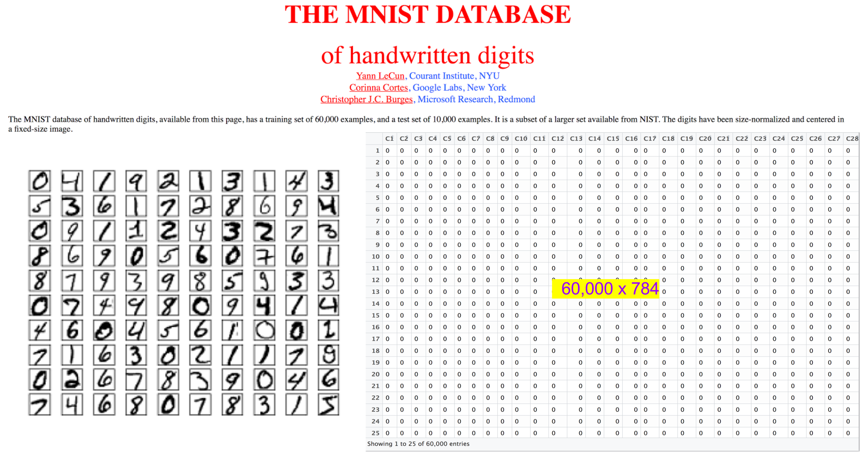
16.53. Another Canonical Example: Digit Recognition (MNIST)#
Extensible to many finance prediction problems.
Information set: 784 (28 x 28) pixels for category prediction.
Would you run a multinomial regression on these 784 columns.
https://www.cs.toronto.edu/~kriz/cifar.html
Image("NLP_images/MNIST.png", width=800)
## Read in the data set
train = pd.read_csv("NLP_data/train.csv", header=None)
test = pd.read_csv("NLP_data/test.csv", header=None)
print(shape(train))
print(shape(test))
(60000, 785)
(10000, 785)
## Reformat the data
X_train = train.loc[:,:783]
Y_train = train.loc[:,784]
print(shape(X_train))
print(shape(Y_train))
X_test = test.loc[:,:783]
Y_test = test.loc[:,784]
print(shape(X_test))
print(shape(Y_test))
y.labels = to_categorical(Y_train, num_classes=10)
print(shape(y.labels))
print(y.labels[1:5,:])
print(Y_train[1:5])
(60000, 784)
(60000,)
(10000, 784)
(10000,)
(60000, 10)
[[0. 0. 0. 1. 0. 0. 0. 0. 0. 0.]
 [1. 0. 0. 0. 0. 0. 0. 0. 0. 0.]
 [1. 0. 0. 0. 0. 0. 0. 0. 0. 0.]
 [0. 0. 1. 0. 0. 0. 0. 0. 0. 0.]]
1    3
2    0
3    0
4    2
Name: 784, dtype: int64
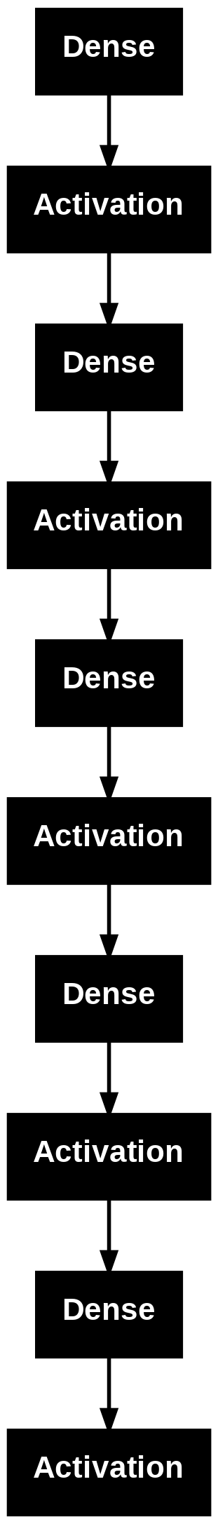
## Define the neural net and compile it
from keras.models import Sequential
from keras.layers import Dense, Activation, Dropout
# from keras.optimizers import SGD
from tensorflow.keras.utils import plot_model

data_dim = shape(X_train)[1]

model = Sequential([
    Dense(100, input_shape=(784,)),
    Activation('sigmoid'),
    Dense(100),
    Activation('sigmoid'),
    Dense(100),
    Activation('sigmoid'),
    Dense(100),
    Activation('sigmoid'),
    Dense(10),
    Activation('softmax'),
])

#model = Sequential()
#model.add(Dense(100, activation='sigmoid', input_dim=data_dim))
#model.add(Dropout(0.25))
#model.add(Dense(100, activation='sigmoid'))
#model.add(Dropout(0.25))
#model.add(Dense(100, activation='sigmoid'))
#model.add(Dropout(0.25))
#model.add(Dense(100, activation='sigmoid'))
#model.add(Dropout(0.25))
#model.add(Dense(10, activation='softmax'))

model.compile(optimizer='rmsprop',
              loss='categorical_crossentropy',
              metrics=['accuracy'])
model.summary()
/usr/local/lib/python3.12/dist-packages/keras/src/layers/core/dense.py:93: UserWarning: Do not pass an `input_shape`/`input_dim` argument to a layer. When using Sequential models, prefer using an `Input(shape)` object as the first layer in the model instead.
  super().__init__(activity_regularizer=activity_regularizer, **kwargs)
Model: "sequential_1"
┏━━━━━━━━━━━━━━━━━━━━━━━━━━━━━━━━━┳━━━━━━━━━━━━━━━━━━━━━━━━┳━━━━━━━━━━━━━━━┓
┃ Layer (type)                    ┃ Output Shape           ┃       Param # ┃
┡━━━━━━━━━━━━━━━━━━━━━━━━━━━━━━━━━╇━━━━━━━━━━━━━━━━━━━━━━━━╇━━━━━━━━━━━━━━━┩
│ dense_4 (Dense)                 │ (None, 100)            │        78,500 │
├─────────────────────────────────┼────────────────────────┼───────────────┤
│ activation (Activation)         │ (None, 100)            │             0 │
├─────────────────────────────────┼────────────────────────┼───────────────┤
│ dense_5 (Dense)                 │ (None, 100)            │        10,100 │
├─────────────────────────────────┼────────────────────────┼───────────────┤
│ activation_1 (Activation)       │ (None, 100)            │             0 │
├─────────────────────────────────┼────────────────────────┼───────────────┤
│ dense_6 (Dense)                 │ (None, 100)            │        10,100 │
├─────────────────────────────────┼────────────────────────┼───────────────┤
│ activation_2 (Activation)       │ (None, 100)            │             0 │
├─────────────────────────────────┼────────────────────────┼───────────────┤
│ dense_7 (Dense)                 │ (None, 100)            │        10,100 │
├─────────────────────────────────┼────────────────────────┼───────────────┤
│ activation_3 (Activation)       │ (None, 100)            │             0 │
├─────────────────────────────────┼────────────────────────┼───────────────┤
│ dense_8 (Dense)                 │ (None, 10)             │         1,010 │
├─────────────────────────────────┼────────────────────────┼───────────────┤
│ activation_4 (Activation)       │ (None, 10)             │             0 │
└─────────────────────────────────┴────────────────────────┴───────────────┘
Total params: 109,810 (428.95 KB)
Trainable params: 109,810 (428.95 KB)
Non-trainable params: 0 (0.00 B)
%%capture
!pip install pydot
!pip install graphviz
plot_model(model)
## Fit/train the model (x,y need to be matrices)
model.fit(X_train, y.labels, epochs=10, batch_size=32, verbose=2, validation_split=0.2)
Epoch 1/10
1500/1500 - 6s - 4ms/step - accuracy: 0.7326 - loss: 0.8534 - val_accuracy: 0.8553 - val_loss: 0.4897
Epoch 2/10
1500/1500 - 4s - 3ms/step - accuracy: 0.8838 - loss: 0.3996 - val_accuracy: 0.8972 - val_loss: 0.3498
Epoch 3/10
1500/1500 - 4s - 3ms/step - accuracy: 0.9046 - loss: 0.3234 - val_accuracy: 0.9078 - val_loss: 0.3071
Epoch 4/10
1500/1500 - 4s - 2ms/step - accuracy: 0.9154 - loss: 0.2842 - val_accuracy: 0.9128 - val_loss: 0.2915
Epoch 5/10
1500/1500 - 5s - 3ms/step - accuracy: 0.9219 - loss: 0.2603 - val_accuracy: 0.9233 - val_loss: 0.2607
Epoch 6/10
1500/1500 - 6s - 4ms/step - accuracy: 0.9253 - loss: 0.2466 - val_accuracy: 0.9263 - val_loss: 0.2375
Epoch 7/10
1500/1500 - 7s - 5ms/step - accuracy: 0.9306 - loss: 0.2296 - val_accuracy: 0.9318 - val_loss: 0.2301
Epoch 8/10
1500/1500 - 9s - 6ms/step - accuracy: 0.9345 - loss: 0.2138 - val_accuracy: 0.9298 - val_loss: 0.2309
Epoch 9/10
1500/1500 - 8s - 5ms/step - accuracy: 0.9340 - loss: 0.2132 - val_accuracy: 0.9328 - val_loss: 0.2193
Epoch 10/10
1500/1500 - 9s - 6ms/step - accuracy: 0.9370 - loss: 0.2065 - val_accuracy: 0.9378 - val_loss: 0.2123
<keras.src.callbacks.history.History at 0x7b50ec08b140>
## In Sample
yhat = model.predict(X_train, batch_size=32)
yhat = [argmax(j) for j in yhat]

## Confusion matrix
from sklearn.metrics import confusion_matrix
cm = confusion_matrix(yhat,Y_train)
print(" ")
print(cm)

##
acc = sum(diag(cm))/len(Y_train)
print("Accuracy = ",acc)
1875/1875 ━━━━━━━━━━━━━━━━━━━━ 7s 3ms/step

[[5712    0   26    7   10   24   54    7   19   21]
 [   0 6521   11    8   13    8    8   16   51   11]
 [  31   36 5587   84   43   22   27   36   39   10]
 [  13   56  126 5715    2  178    4   39  110   65]
 [   5    3   29    0 5210    5   20   25    5   62]
 [  40   20   23  121   19 5017  118   16   96   43]
 [  17    3   22   10   26   36 5651    0   21    0]
 [   5   18   55   59   18    9    0 5980    6   91]
 [  75   68   65   87   48   81   32   14 5428   74]
 [  25   17   14   40  453   41    4  132   76 5572]]
Accuracy =  0.9398833333333333
## Out of Sample
yhat = model.predict(X_test, batch_size=32)
yhat = [argmax(j) for j in yhat]

## Confusion matrix
from sklearn.metrics import confusion_matrix
cm = confusion_matrix(yhat,Y_test)
print(" ")
print(cm)

##
acc = sum(diag(cm))/len(Y_test)
print("Accuracy = ",acc)
313/313 ━━━━━━━━━━━━━━━━━━━━ 1s 4ms/step

[[ 948    0    9    0    2    8   17    1    6    5]
 [   0 1116    0    0    0    1    1    6    2    6]
 [   6    1  966   13   11    1    8   19    4    0]
 [   3    6   16  950    0   37    3    8   17   13]
 [   0    0    6    0  875    0    2    2    4   17]
 [   5    1    7   12    2  812   19    1   14   11]
 [   4    2    2    0    3    8  901    0    9    0]
 [   6    0    9   13    7    2    0  962    4    8]
 [   6    9   12   18    8   15    6    1  905   10]
 [   2    0    5    4   74    8    1   28    9  939]]
Accuracy =  0.9374
16.54. Adversarial Models#
To see adversarial models, try: https://kennysong.github.io/adversarial.js/
16.55. Image Processing, Transfer Learning#
Slides on Image Processing using Deep Learning by Subir Varma: https://drive.google.com/file/d/19xPCf2M66Dws06XxXLgEhuqJFiKmUEJ1/view?usp=sharing
Image processing with transfer learning: https://drive.google.com/file/d/1D3Cg288wVY-e5BHuDNHec3wd-LStflMr/view?usp=sharing. From: Practical Deep Learning for Cloud and Mobile (O’Reilly) by Anirudh Koul, Siddha Ganju & Meher Kasam.
Recognizing Images using NNs: https://drive.google.com/file/d/1OMQOZuEmnw0Kxvo5O1C9kf6mbQnPXYvj/view?usp=sharing. (Build your first Convolutional Neural Network to recognize images: A step-by-step guide to building your own image recognition software with Convolutional Neural Networks using Keras on CIFAR-10 images! by Joseph Lee Wei En.): https://medium.com/intuitive-deep-learning/build-your-first-convolutional-neural-network-to-recognize-images-84b9c78fe0ce
16.56. Learning the Black-Scholes Equation#
See : Hutchinson, Lo, Poggio (1994)
from scipy.stats import norm
def BSM(S,K,T,sig,rf,dv,cp):  #cp = {+1.0 (calls), -1.0 (puts)}
    d1 = (math.log(S/K)+(rf-dv+0.5*sig**2)*T)/(sig*math.sqrt(T))
    d2 = d1 - sig*math.sqrt(T)
    return cp*S*math.exp(-dv*T)*norm.cdf(d1*cp) - cp*K*math.exp(-rf*T)*norm.cdf(d2*cp)

df = pd.read_csv('NLP_data/BS_training.csv')
16.57. Normalizing spot and call prices#
\(C\) is homogeneous degree one, so $\( aC(S,K) = C(aS,aK) \)\( This means we can normalize spot and call prices and remove a variable by dividing by \)K\(. \)\( \frac{C(S,K)}{K} = C(S/K,1) \)$
df['Stock Price'] = df['Stock Price']/df['Strike Price']
df['Call Price']  = df['Call Price'] /df['Strike Price']
16.58. Data, libraries, activation functions#
n = 300000
n_train =  (int)(0.8 * n)
train = df[0:n_train]
X_train = train[['Stock Price', 'Maturity', 'Dividends', 'Volatility', 'Risk-free']].values
y_train = train['Call Price'].values
test = df[n_train+1:n]
X_test = test[['Stock Price', 'Maturity', 'Dividends', 'Volatility', 'Risk-free']].values
y_test = test['Call Price'].values
#Import libraries
import numpy as np
from keras.models import Sequential
from keras.layers import Dense, Dropout, Activation, LeakyReLU
import tensorflow as tf

def custom_activation(x):
    return tf.math.exp(x)
16.59. Set up, compile and fit the model#
nodes = 120
model = Sequential()

model.add(Dense(nodes, input_dim=X_train.shape[1]))
#model.add("relu")
model.add(Dropout(0.25))

model.add(Dense(nodes, activation='elu'))
model.add(Dropout(0.25))

model.add(Dense(nodes, activation='relu'))
model.add(Dropout(0.25))

model.add(Dense(nodes, activation='elu'))
model.add(Dropout(0.25))

model.add(Dense(1))
model.add(Activation(custom_activation))

model.compile(loss='mse',optimizer='rmsprop')

model.fit(X_train, y_train, batch_size=64, epochs=10, validation_split=0.1, verbose=2)
Epoch 1/10
/usr/local/lib/python3.12/dist-packages/keras/src/layers/core/dense.py:93: UserWarning: Do not pass an `input_shape`/`input_dim` argument to a layer. When using Sequential models, prefer using an `Input(shape)` object as the first layer in the model instead.
  super().__init__(activity_regularizer=activity_regularizer, **kwargs)
3375/3375 - 12s - 3ms/step - loss: 0.0055 - val_loss: 7.7318e-04
Epoch 2/10
3375/3375 - 9s - 3ms/step - loss: 0.0015 - val_loss: 8.9263e-04
Epoch 3/10
3375/3375 - 8s - 2ms/step - loss: 0.0012 - val_loss: 2.4795e-04
Epoch 4/10
3375/3375 - 8s - 2ms/step - loss: 0.0010 - val_loss: 2.9479e-04
Epoch 5/10
3375/3375 - 8s - 2ms/step - loss: 9.4735e-04 - val_loss: 5.8266e-04
Epoch 6/10
3375/3375 - 8s - 2ms/step - loss: 8.7909e-04 - val_loss: 3.1445e-04
Epoch 7/10
3375/3375 - 8s - 3ms/step - loss: 8.2551e-04 - val_loss: 1.8766e-04
Epoch 8/10
3375/3375 - 8s - 2ms/step - loss: 7.8673e-04 - val_loss: 2.2394e-04
Epoch 9/10
3375/3375 - 8s - 3ms/step - loss: 7.5580e-04 - val_loss: 2.3692e-04
Epoch 10/10
3375/3375 - 8s - 2ms/step - loss: 7.3113e-04 - val_loss: 1.4039e-04
<keras.src.callbacks.history.History at 0x79a27e508e30>
model.summary()
Model: "sequential_2"
┏━━━━━━━━━━━━━━━━━━━━━━━━━━━━━━━━━┳━━━━━━━━━━━━━━━━━━━━━━━━┳━━━━━━━━━━━━━━━┓
┃ Layer (type)                    ┃ Output Shape           ┃       Param # ┃
┡━━━━━━━━━━━━━━━━━━━━━━━━━━━━━━━━━╇━━━━━━━━━━━━━━━━━━━━━━━━╇━━━━━━━━━━━━━━━┩
│ dense_9 (Dense)                 │ (None, 120)            │           720 │
├─────────────────────────────────┼────────────────────────┼───────────────┤
│ dropout (Dropout)               │ (None, 120)            │             0 │
├─────────────────────────────────┼────────────────────────┼───────────────┤
│ dense_10 (Dense)                │ (None, 120)            │        14,520 │
├─────────────────────────────────┼────────────────────────┼───────────────┤
│ dropout_1 (Dropout)             │ (None, 120)            │             0 │
├─────────────────────────────────┼────────────────────────┼───────────────┤
│ dense_11 (Dense)                │ (None, 120)            │        14,520 │
├─────────────────────────────────┼────────────────────────┼───────────────┤
│ dropout_2 (Dropout)             │ (None, 120)            │             0 │
├─────────────────────────────────┼────────────────────────┼───────────────┤
│ dense_12 (Dense)                │ (None, 120)            │        14,520 │
├─────────────────────────────────┼────────────────────────┼───────────────┤
│ dropout_3 (Dropout)             │ (None, 120)            │             0 │
├─────────────────────────────────┼────────────────────────┼───────────────┤
│ dense_13 (Dense)                │ (None, 1)              │           121 │
├─────────────────────────────────┼────────────────────────┼───────────────┤
│ activation_5 (Activation)       │ (None, 1)              │             0 │
└─────────────────────────────────┴────────────────────────┴───────────────┘
Total params: 88,804 (346.89 KB)
Trainable params: 44,401 (173.44 KB)
Non-trainable params: 0 (0.00 B)
Optimizer params: 44,403 (173.45 KB)
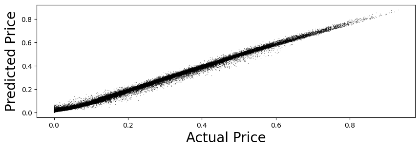
def CheckAccuracy(y,y_hat):
stats = dict()
stats['diff'] = y - y_hat
stats['mse'] = mean(stats['diff']**2)
print("Mean Squared Error: ", stats['mse'])
stats['rmse'] = sqrt(stats['mse'])
print("Root Mean Squared Error: ", stats['rmse'])
stats['mae'] = mean(abs(stats['diff']))
print("Mean Absolute Error: ", stats['mae'])
stats['mpe'] = sqrt(stats['mse'])/mean(y)
print("Mean Percent Error: ", stats['mpe'])
#plots
mpl.rcParams['agg.path.chunksize'] = 100000
figure(figsize=(10,3))
plt.scatter(y, y_hat,color='black',linewidth=0.3,alpha=0.4, s=0.5)
plt.xlabel('Actual Price',fontsize=20,fontname='Times New Roman')
plt.ylabel('Predicted Price',fontsize=20,fontname='Times New Roman')
plt.show()
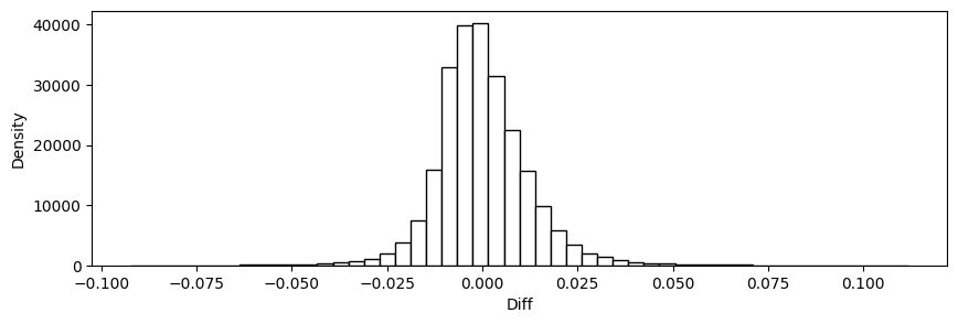
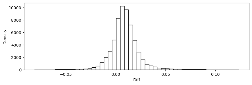
figure(figsize=(10,3))
plt.hist(stats['diff'], bins=50,edgecolor='black',color='white')
plt.xlabel('Diff')
plt.ylabel('Density')
plt.show()
return stats
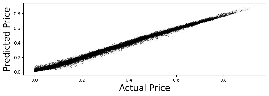
16.60. Predict and check accuracy (in-sample)#
y_train_hat = model.predict(X_train)
#reduce dim (240000,1) -> (240000,) to match y_train's dim
y_train_hat = squeeze(y_train_hat)
CheckAccuracy(y_train, y_train_hat)
7500/7500 ━━━━━━━━━━━━━━━━━━━━ 11s 1ms/step
WARNING:matplotlib.font_manager:findfont: Font family 'Times New Roman' not found.
WARNING:matplotlib.font_manager:findfont: Font family 'Times New Roman' not found.
WARNING:matplotlib.font_manager:findfont: Font family 'Times New Roman' not found.
WARNING:matplotlib.font_manager:findfont: Font family 'Times New Roman' not found.
WARNING:matplotlib.font_manager:findfont: Font family 'Times New Roman' not found.
WARNING:matplotlib.font_manager:findfont: Font family 'Times New Roman' not found.
WARNING:matplotlib.font_manager:findfont: Font family 'Times New Roman' not found.
WARNING:matplotlib.font_manager:findfont: Font family 'Times New Roman' not found.
Mean Squared Error:       0.00014354266244062555
Root Mean Squared Error:  0.01198092911424759
Mean Absolute Error:      0.008734802954738614
Mean Percent Error:       0.04478733371495744
{'diff': array([ 0.00217092, -0.0043095 ,  0.00295363, ...,  0.00624732,
         0.00106334, -0.00882631]),
 'mse': np.float64(0.00014354266244062555),
 'rmse': np.float64(0.01198092911424759),
 'mae': np.float64(0.008734802954738614),
 'mpe': np.float64(0.04478733371495744)}
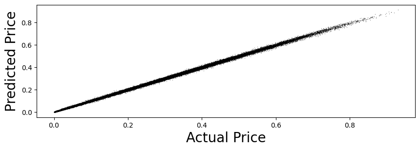
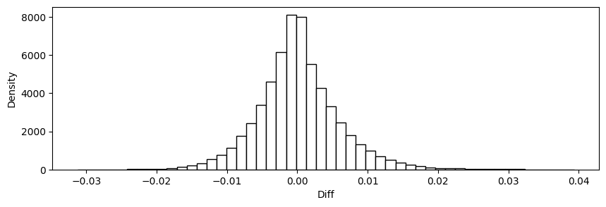
16.61. Predict and check accuracy (validation-sample)#
y_test_hat = model.predict(X_test)
y_test_hat = squeeze(y_test_hat)
test_stats = CheckAccuracy(y_test, y_test_hat)
1875/1875 ━━━━━━━━━━━━━━━━━━━━ 3s 1ms/step
WARNING:matplotlib.font_manager:findfont: Font family 'Times New Roman' not found.
WARNING:matplotlib.font_manager:findfont: Font family 'Times New Roman' not found.
WARNING:matplotlib.font_manager:findfont: Font family 'Times New Roman' not found.
WARNING:matplotlib.font_manager:findfont: Font family 'Times New Roman' not found.
WARNING:matplotlib.font_manager:findfont: Font family 'Times New Roman' not found.
WARNING:matplotlib.font_manager:findfont: Font family 'Times New Roman' not found.
WARNING:matplotlib.font_manager:findfont: Font family 'Times New Roman' not found.
WARNING:matplotlib.font_manager:findfont: Font family 'Times New Roman' not found.
Mean Squared Error:       0.00024734096163625346
Root Mean Squared Error:  0.01572707733929777
Mean Absolute Error:      0.011981657814608197
Mean Percent Error:       0.05887565394485396
16.62. Random Forest of decision trees#
A Random Forest uses several decision trees to make hypotheses about regions within subsamples of the data, then makes predictions based on the majority vote of these trees. This safeguards against overfitting/memorization of the training data.
16.63. Prepare Data#
n = 300000
n_train =  (int)(0.8 * n)
train = df[0:n_train]
X_train = train[['Stock Price', 'Maturity', 'Dividends', 'Volatility', 'Risk-free']].values
y_train = train['Call Price'].values
test = df[n_train+1:n]
X_test = test[['Stock Price', 'Maturity', 'Dividends', 'Volatility', 'Risk-free']].values
y_test = test['Call Price'].values
16.64. Fit Random Forest#
%%time
from sklearn.ensemble import RandomForestRegressor

forest = RandomForestRegressor()
forest = forest.fit(X_train, y_train)
y_test_hat = forest.predict(X_test)
CPU times: user 3min 54s, sys: 1.72 s, total: 3min 56s
Wall time: 4min 25s
stats = CheckAccuracy(y_test, y_test_hat)
WARNING:matplotlib.font_manager:findfont: Font family 'Times New Roman' not found.
WARNING:matplotlib.font_manager:findfont: Font family 'Times New Roman' not found.
WARNING:matplotlib.font_manager:findfont: Font family 'Times New Roman' not found.
WARNING:matplotlib.font_manager:findfont: Font family 'Times New Roman' not found.
WARNING:matplotlib.font_manager:findfont: Font family 'Times New Roman' not found.
WARNING:matplotlib.font_manager:findfont: Font family 'Times New Roman' not found.
WARNING:matplotlib.font_manager:findfont: Font family 'Times New Roman' not found.
WARNING:matplotlib.font_manager:findfont: Font family 'Times New Roman' not found.
Mean Squared Error:       3.441939992235234e-05
Root Mean Squared Error:  0.005866804915995788
Mean Absolute Error:      0.004273785915686731
Mean Percent Error:       0.02196288404667812
16.65. Use the same approach with text#
Convert the text into a vector (embedding) using any vectorization/transformer approach.
Use deep learning to train and test the model on the text embeddings.
# Read data
df = pd.read_csv('NLP_data/Sentences_AllAgree.txt', sep=".@", header=None, engine='python', encoding = "ISO-8859-1")  # Finbert data
# df = pd.read_csv('NLP_data/Sentences_AllAgree.txt', sep=".@", header=None, engine='python', encoding = "utf-8")  # Finbert data
# tmp = pd.read_csv('NLP_data/Sentences_75Agree.txt', sep=".@", header=None, engine='python')
# df = pd.concat([df,tmp])
# tmp = pd.read_csv('NLP_data/Sentences_66Agree.txt', sep=".@", header=None, engine='python')
# df = pd.concat([df,tmp])
# tmp = pd.read_csv('NLP_data/Sentences_50Agree.txt', sep=".@", header=None, engine='python')
# df = pd.concat([df,tmp])
df.columns = ["Text","Label"]
print(df.shape)
df.head()
(2264, 2)
| Text | Label | |
|---|---|---|
| 0 | According to Gran , the company has no plans t... | neutral |
| 1 | For the last quarter of 2010 , Componenta 's n... | positive |
| 2 | In the third quarter of 2010 , net sales incre... | positive |
| 3 | Operating profit rose to EUR 13.1 mn from EUR ... | positive |
| 4 | Operating profit totalled EUR 21.1 mn , up fro... | positive |
from transformers import AutoTokenizer, AutoModel
import torch

# Load pre-trained BERT model and tokenizer
model_name = 'bert-base-uncased'  # You can choose a different BERT model here
tokenizer = AutoTokenizer.from_pretrained(model_name)
model = AutoModel.from_pretrained(model_name)

def get_bert_embedding(text):
    # Tokenize the input text
    inputs = tokenizer(text, return_tensors='pt', truncation=True, padding=True)
    # Get BERT embeddings
    with torch.no_grad():
        outputs = model(**inputs)
        embeddings = outputs.last_hidden_state
        # Extract the embedding for the [CLS] token (often used as sentence embedding)
        sentence_embedding = embeddings[:, 0, :]
        return sentence_embedding.numpy()

# Input sentence
sentence = "This is an example sentence."

# Print the embedding
e = get_bert_embedding(sentence)[0]
print(len(e))
# print(e)
/usr/local/lib/python3.12/dist-packages/huggingface_hub/utils/_auth.py:94: UserWarning:
The secret `HF_TOKEN` does not exist in your Colab secrets.
To authenticate with the Hugging Face Hub, create a token in your settings tab (https://huggingface.co/settings/tokens), set it as secret in your Google Colab and restart your session.
You will be able to reuse this secret in all of your notebooks.
Please note that authentication is recommended but still optional to access public models or datasets.
  warnings.warn(
768
%%time
train_list = list(df.Text)
n = len(train_list)
vecs = zeros((len(train_list),768))
for j in range(200):
  sentences = [train_list[j]]
  vectors_bert = get_bert_embedding(sentences)
  vecs[j,:] = np.array(vectors_bert)
  train_list.remove(train_list[j])

print(vecs.shape)
vecs = vecs[:200,:]
vecs.shape
(2264, 768)
CPU times: user 28.6 s, sys: 19.6 ms, total: 28.6 s
Wall time: 28.8 s
(200, 768)
df.Label
| Label | |
|---|---|
| 0 | neutral |
| 1 | positive |
| 2 | positive |
| 3 | positive |
| 4 | positive |
| ... | ... |
| 2259 | negative |
| 2260 | negative |
| 2261 | negative |
| 2262 | negative |
| 2263 | negative |
2264 rows × 1 columns
## Make label data have 1-shape, 1=malignant
from keras.utils import to_categorical
from keras.models import Sequential
from keras.layers import Dense, Activation

X_data = vecs
print("X Dataset size =", X_data.shape)

# y_data = zeros(len(df.Label))
y_data = zeros(200)
for j in range(len(y_data)):
  if df.Label[j]=='positive':
    y_data[j] = 1
  if df.Label[j]=='negative':
    y_data[j] = -1

y_data = to_categorical(y_data, num_classes=3)
print(y_data[:5])
print(y_data.shape)
X Dataset size = (200, 768)
[[1. 0. 0.]
 [0. 1. 0.]
 [0. 1. 0.]
 [0. 1. 0.]
 [0. 1. 0.]]
(200, 3)
nodes = 128
model = Sequential([
    Dense(nodes, input_shape=(768,)),
    Activation('sigmoid'),
    Dense(nodes),
    Activation('sigmoid'),
    Dense(nodes),
    Activation('sigmoid'),
    Dense(nodes),
    Activation('sigmoid'),
    Dense(3),
    Activation('softmax'),
])

model.compile(optimizer='rmsprop',
              loss='categorical_crossentropy',
              metrics=['accuracy'])
model.summary()
/usr/local/lib/python3.12/dist-packages/keras/src/layers/core/dense.py:93: UserWarning: Do not pass an `input_shape`/`input_dim` argument to a layer. When using Sequential models, prefer using an `Input(shape)` object as the first layer in the model instead.
  super().__init__(activity_regularizer=activity_regularizer, **kwargs)
Model: "sequential_3"
┏━━━━━━━━━━━━━━━━━━━━━━━━━━━━━━━━━┳━━━━━━━━━━━━━━━━━━━━━━━━┳━━━━━━━━━━━━━━━┓
┃ Layer (type)                    ┃ Output Shape           ┃       Param # ┃
┡━━━━━━━━━━━━━━━━━━━━━━━━━━━━━━━━━╇━━━━━━━━━━━━━━━━━━━━━━━━╇━━━━━━━━━━━━━━━┩
│ dense_14 (Dense)                │ (None, 128)            │        98,432 │
├─────────────────────────────────┼────────────────────────┼───────────────┤
│ activation_6 (Activation)       │ (None, 128)            │             0 │
├─────────────────────────────────┼────────────────────────┼───────────────┤
│ dense_15 (Dense)                │ (None, 128)            │        16,512 │
├─────────────────────────────────┼────────────────────────┼───────────────┤
│ activation_7 (Activation)       │ (None, 128)            │             0 │
├─────────────────────────────────┼────────────────────────┼───────────────┤
│ dense_16 (Dense)                │ (None, 128)            │        16,512 │
├─────────────────────────────────┼────────────────────────┼───────────────┤
│ activation_8 (Activation)       │ (None, 128)            │             0 │
├─────────────────────────────────┼────────────────────────┼───────────────┤
│ dense_17 (Dense)                │ (None, 128)            │        16,512 │
├─────────────────────────────────┼────────────────────────┼───────────────┤
│ activation_9 (Activation)       │ (None, 128)            │             0 │
├─────────────────────────────────┼────────────────────────┼───────────────┤
│ dense_18 (Dense)                │ (None, 3)              │           387 │
├─────────────────────────────────┼────────────────────────┼───────────────┤
│ activation_10 (Activation)      │ (None, 3)              │             0 │
└─────────────────────────────────┴────────────────────────┴───────────────┘
Total params: 148,355 (579.51 KB)
Trainable params: 148,355 (579.51 KB)
Non-trainable params: 0 (0.00 B)
## Fit/train the model (x,y need to be matrices)
model.fit(X_data, y_data, epochs=5, batch_size=32, verbose=2, validation_split=0.2)
Epoch 1/5
5/5 - 2s - 461ms/step - accuracy: 0.9688 - loss: 0.4498 - val_accuracy: 1.0000 - val_loss: 0.1156
Epoch 2/5
5/5 - 0s - 15ms/step - accuracy: 0.9688 - loss: 0.1768 - val_accuracy: 1.0000 - val_loss: 0.0620
Epoch 3/5
5/5 - 0s - 14ms/step - accuracy: 0.9688 - loss: 0.1622 - val_accuracy: 1.0000 - val_loss: 0.0445
Epoch 4/5
5/5 - 0s - 14ms/step - accuracy: 0.9688 - loss: 0.1502 - val_accuracy: 1.0000 - val_loss: 0.0427
Epoch 5/5
5/5 - 0s - 14ms/step - accuracy: 0.9688 - loss: 0.1497 - val_accuracy: 1.0000 - val_loss: 0.0355
<keras.src.callbacks.history.History at 0x79a16288df10>
16.66. Relevant Applications#
Big Data and ML/AI in Central Banking: IFC Bulletin No 50 The use of big data analytics and artificial intelligence in central banking Proceedings of the IFC, Bank Indonesia International Workshop and Seminar in Bali on 23-26 July, 2018 (published May 2019): https://www.bis.org/ifc/publ/ifcb50.pdf;
https://drive.google.com/file/d/1at-baZON-GfL7MuPcQC0EyJCskiF7rUl/view?usp=sharing
16.67. Causal Models#
Deep Learning, specifically, and machine learning, more generally, has been criticized by econometricians as being weaker than causal models. That is, correlation is not causality. Here is an article about a recent development in taking NNs in the direction of causal models: https://medium.com/mit-technology-review/deep-learning-could-reveal-why-the-world-works-the-way-it-does-9be8b5fbfe4f; https://drive.google.com/file/d/1r4UPFQQv-vutQXdlmpmCyB9_nO14FZMe/view?usp=sharing
16.68. Recap Video#
You can watch an excellent video from MIT to get a recap of all the topics discussed above: https://youtu.be/7sB052Pz0sQ