
29. Dimension Reduction (and Topics)#
Squeezing the data down to be digested easily for modeling and analysis.
from google.colab import drive
drive.mount('/content/drive')  # Add My Drive/<>

import os
os.chdir('drive/My Drive')
os.chdir('Books_Writings/NLPBook/')
Mounted at /content/drive
%%capture
%pylab inline
import pandas as pd
import os
%load_ext rpy2.ipython
from IPython.display import Image
29.1. Dimension Reduction of Text#
We show here that documents end up in a space of two PCs (principal components).
LDA is a way of reducing documents into a smaller space.
We can use the wine reviews dataset from Kaggle.
https://www.kaggle.com/thebrownviking20/topic-modelling-with-spacy-and-scikit-learn
%%time
os.system('wget https://github.com/morisasy/kaggle/raw/master/data/winemag-data-130k-v2.csv')
os.system('mv winemag-data-130k-v2.csv NLP_data/')
CPU times: user 25 ms, sys: 3.85 ms, total: 28.8 ms
Wall time: 4.84 s
0
wineDF = pd.read_csv("NLP_data/winemag-data-130k-v2.csv")
print(wineDF.shape)
wineDF.head()
(129971, 14)
| Unnamed: 0 | country | description | designation | points | price | province | region_1 | region_2 | taster_name | taster_twitter_handle | title | variety | winery | |
|---|---|---|---|---|---|---|---|---|---|---|---|---|---|---|
| 0 | 0 | Italy | Aromas include tropical fruit, broom, brimston... | Vulkà Bianco | 87 | NaN | Sicily & Sardinia | Etna | NaN | Kerin O’Keefe | @kerinokeefe | Nicosia 2013 Vulkà Bianco (Etna) | White Blend | Nicosia |
| 1 | 1 | Portugal | This is ripe and fruity, a wine that is smooth... | Avidagos | 87 | 15.0 | Douro | NaN | NaN | Roger Voss | @vossroger | Quinta dos Avidagos 2011 Avidagos Red (Douro) | Portuguese Red | Quinta dos Avidagos |
| 2 | 2 | US | Tart and snappy, the flavors of lime flesh and... | NaN | 87 | 14.0 | Oregon | Willamette Valley | Willamette Valley | Paul Gregutt | @paulgwine | Rainstorm 2013 Pinot Gris (Willamette Valley) | Pinot Gris | Rainstorm |
| 3 | 3 | US | Pineapple rind, lemon pith and orange blossom ... | Reserve Late Harvest | 87 | 13.0 | Michigan | Lake Michigan Shore | NaN | Alexander Peartree | NaN | St. Julian 2013 Reserve Late Harvest Riesling ... | Riesling | St. Julian |
| 4 | 4 | US | Much like the regular bottling from 2012, this... | Vintner's Reserve Wild Child Block | 87 | 65.0 | Oregon | Willamette Valley | Willamette Valley | Paul Gregutt | @paulgwine | Sweet Cheeks 2012 Vintner's Reserve Wild Child... | Pinot Noir | Sweet Cheeks |
from sklearn.decomposition import NMF, LatentDirichletAllocation, TruncatedSVD
from sklearn.feature_extraction.text import CountVectorizer
from sklearn.manifold import TSNE
from tqdm import tqdm
import string
%%capture
!pip install spacy
import spacy
from spacy.lang.en.stop_words import STOP_WORDS
from spacy.lang.en import English
!python -m spacy download en_core_web_sm
# Load in the spaCy object, i.e., the language model
nlp = spacy.load('en_core_web_sm')
wineDF.description
| description | |
|---|---|
| 0 | Aromas include tropical fruit, broom, brimston... |
| 1 | This is ripe and fruity, a wine that is smooth... |
| 2 | Tart and snappy, the flavors of lime flesh and... |
| 3 | Pineapple rind, lemon pith and orange blossom ... |
| 4 | Much like the regular bottling from 2012, this... |
| ... | ... |
| 129966 | Notes of honeysuckle and cantaloupe sweeten th... |
| 129967 | Citation is given as much as a decade of bottl... |
| 129968 | Well-drained gravel soil gives this wine its c... |
| 129969 | A dry style of Pinot Gris, this is crisp with ... |
| 129970 | Big, rich and off-dry, this is powered by inte... |
129971 rows × 1 columns
# Functions to parse the reviews
punctuations = string.punctuation
stopwords = list(STOP_WORDS)

parser = English()
def spacy_tokenizer(sentence):
    mytokens = list(parser(sentence))
#     mytokens = [word.lemma_.lower().strip() if word.lemma_ != "-PRON-" else word.lower_ for word in mytokens ]
    mytokens = [word.lower_ for word in mytokens ]
    mytokens = [word for word in mytokens if word not in stopwords and word not in punctuations ]
    mytokens = " ".join([i for i in mytokens])
    return mytokens
Let’s use the TQDM progress bar. The abbreviation tqdm has interesting naming origins: https://tqdm.github.io
%%time
tqdm.pandas()
wineDF["processed_description"] = wineDF["description"].progress_apply(spacy_tokenizer)
100%|██████████| 129971/129971 [01:12<00:00, 1794.82it/s]
CPU times: user 55.3 s, sys: 586 ms, total: 55.9 s
Wall time: 1min 12s
for j in range(5):
    print(wineDF.processed_description[j])
aromas include tropical fruit broom brimstone dried herb palate overly expressive offering unripened apple citrus dried sage alongside brisk acidity
ripe fruity wine smooth structured firm tannins filled juicy red berry fruits freshened acidity   drinkable certainly better 2016
tart snappy flavors lime flesh rind dominate green pineapple pokes crisp acidity underscoring flavors wine stainless steel fermented
pineapple rind lemon pith orange blossom start aromas palate bit opulent notes honey drizzled guava mango giving way slightly astringent semidry finish
like regular bottling 2012 comes rough tannic rustic earthy herbal characteristics nonetheless think pleasantly unfussy country wine good companion hearty winter stew
# Create the document-term matrix
vectorizer = CountVectorizer(min_df=5, max_df=0.9, stop_words='english', lowercase=True, token_pattern='[a-zA-Z\-][a-zA-Z\-]{2,}')
DTM = vectorizer.fit_transform(wineDF["processed_description"])
DTM
<129971x11917 sparse matrix of type '<class 'numpy.int64'>'
	with 2953416 stored elements in Compressed Sparse Row format>
29.2. Topics from LDA using scikit-learn#
Next we use spaCy to fit the LDA model. This is slow and so we run only a few iterations, and the best results will come after many iterations.
%%time
# ~<1 minute per iteration
# Fit LDA in spaCy
n_topics = 3
lda = LatentDirichletAllocation(n_components=n_topics, max_iter=5, learning_method='online',verbose=True)
data_lda = lda.fit_transform(DTM)
iteration: 1 of max_iter: 5
iteration: 2 of max_iter: 5
iteration: 3 of max_iter: 5
iteration: 4 of max_iter: 5
iteration: 5 of max_iter: 5
CPU times: user 3min 2s, sys: 1.39 s, total: 3min 3s
Wall time: 3min 6s
# Functions for printing keywords for each topic
def selected_topics(model, vectorizer, top_n=10):
    for idx, topic in enumerate(model.components_):
        print("Topic %d:" % (idx))
        print([(vectorizer.get_feature_names_out()[i], topic[i])
                        for i in topic.argsort()[:-top_n - 1:-1]])
selected_topics(lda, vectorizer)
Topic 0:
[('flavors', 20950.67018477242), ('wine', 16635.82545843346), ('palate', 16354.406381362307), ('acidity', 15506.05593080573), ('finish', 14769.111553817538), ('fruit', 13941.560939821009), ('apple', 13566.236570759675), ('aromas', 13122.03875126582), ('crisp', 12684.586526258352), ('citrus', 11662.251281882267)]
Topic 1:
[('wine', 55565.60958002671), ('flavors', 27153.00418436964), ('drink', 21554.66699850035), ('fruit', 20633.16021614574), ('ripe', 16809.443714251152), ('acidity', 16485.57645214745), ('tannins', 15305.53765344409), ('rich', 14543.343787563213), ('fruits', 13144.847668129269), ('red', 9631.062687215997)]
Topic 2:
[('aromas', 26374.091755743342), ('cherry', 25480.441094742815), ('palate', 22273.87156641139), ('black', 20613.840965534495), ('tannins', 15636.192367999198), ('finish', 15518.815192377546), ('fruit', 15467.455651759687), ('flavors', 14852.499696966233), ('spice', 12117.49492696586), ('red', 11960.038937625673)]
new_review = "This wine terrific aromatic flavor hint berries almonds lingering aftertaste. Both winter and spring varietals."
text = spacy_tokenizer(new_review)
vec = lda.transform(vectorizer.transform([text]))[0]
print("Topic vector score=",vec)
print("Topic ordering:",argsort(vec)[::-1])
Topic vector score= [0.60990689 0.35577218 0.03432093]
Topic ordering: [0 1 2]
vocab = vectorizer.get_feature_names_out()
vocab
array(['-georges', 'aaron', 'abacela', ..., 'zonin', 'zucchini',
       'zweigelt'], dtype=object)
So, now we are ready and in a position to see how we reduce the dimension of the corpus.
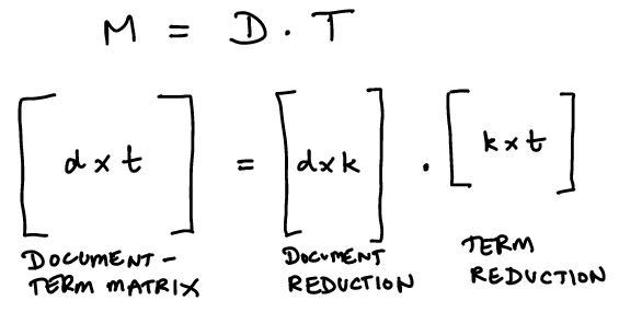
Note that the document-term matrix \(M\) can be reduced to a decomposition using matrix factorization. \(M\) is of dimension \(d \times t\), where \(d\) is the number of documents and \(t\) is the number of terms.
We set \(M = D \cdot T\), where \(D \in {R}^{d \times k}\), where \(k\) is the number of topics.
\(T \in {R}^{k \times t}\).
We can think of this as projecting the documents onto a smaller set of topics instead of terms, i.e., \(k \ll d\).
We can think of this as projecting the terms onto a smaller set of topics, i.e., \(k \ll t\).
Image("NLP_images/DTM_reduction.png", width=500)
# Check for dimension reduction
data_lda.shape
(129971, 3)
lda.perplexity(DTM)
962.4460528706168
29.3. Non-Negative Matrix Factorization (NMF)#
As noted above we are looking to decompose the DTM \(M\) into \(D \cdot T\), with common dimension of size \(k\).
We apply the Froebenius norm:
Let the gradient be \(\nabla f\).
We minimize \(f\) by iteration. First, hold \(T\) fixed and find the best \(D\), then hold \(D\) fixed and find the best \(T\).
If we hold \(T\) fixed, and differentiate with respect to a specific \(d\): \(\nabla f_d = \frac{\partial f}{\partial d} \sum_d \sum_t (M_{dt}^2 - 2 M_{dt} D_{dt} T_{dt} + D_{dt}^2 T_{dt}^2) = 0\).
We get that \(\nabla f_d = \sum_t (MT^\top - DTT^\top) = 0\), which implies that
We want to choose the elements of \(D\) such that
The LHS is as close to the RHS as possible
The elements of \(D\) are non-negative, else we are not doing NMF
Using gradients, we set up the algorithm as follows:
We can choose the learning rate \(\eta_D\) in a clever way to make sure that elements of \(D \geq 0\), i.e., \(\eta_D = \frac{D}{DTT^\top}\), the fraction taken elementwise. So, we now get
or, elementwise
This update rule ensures that \(D_{dt} \geq 0, \forall d,t\). Correspondingly, the update rule for the elements of \(T\) is
n_topics = 3
# Non-Negative Matrix Factorization Model
nmf = NMF(n_components=n_topics)
data_nmf = nmf.fit_transform(DTM)
data_nmf.shape
(129971, 3)
we can get more details here: https://srdas.github.io/MLBook2/24_TextAnaytics_Advanced.html#Non-negative-Matrix-Factorization-(NMF)
You can use this reduced-form matrix for document similarity (for example).
# Latent Semantic Indexing Model using Truncated SVD
lsi = TruncatedSVD(n_components=n_topics)
data_lsi = lsi.fit_transform(DTM)
data_lsi.shape
(129971, 3)
More details here: https://srdas.github.io/MLBook2/24_TextAnaytics_Advanced.html#Singular-Value-Decomposition-(SVD)