
32. Generalized Language Models#
Good reference: https://lilianweng.github.io/lil-log/2019/01/31/generalized-language-models.html
Slides: https://docs.google.com/presentation/d/1xhOocjNJ-6YU_jXPJb_Yi0Vloen65QCyM51S7-Dadfk/edit?usp=sharing
Hands On LLMs (book) GitHub: HandsOnLLM/Hands-On-Large-Language-Models
Interviews on the history of the transformer: https://www.quantamagazine.org/when-chatgpt-broke-an-entire-field-an-oral-history-20250430/
# # Use pytorch kernel and install TF, as needed
# !pip install --upgrade torch
# !pip install --upgrade tensorflow
32.1. Classification with Embeddings and BERT#
We can use many approaches as seen earlier. A good summary of classification approaches in various NLP libraries is discussed here: https://towardsdatascience.com/which-is-the-best-nlp-d7965c71ec5f
from google.colab import drive
drive.mount('/content/drive')  # Add My Drive/<>

import os
os.chdir('drive/My Drive')
os.chdir('Books_Writings/NLPBook/')
Mounted at /content/drive
%%capture
%pylab inline
import pandas as pd
import os
import numpy as np
import matplotlib.pyplot as plt
from IPython.display import Image
32.2. Sequence of Classification Approaches#
Various forms of input are possible:
Use a single vector from the TDM for classification of each document. Easy to construct, but lacking context. Input size is fixed. Vocab size is large.
Use a single TFIDF vector. Same as TDM vectors.
Word2Vec. Convert each word in the document into a fixed length vector. Combine vectors into a matrix for the document and this is the input into the classifier. Requires a package like gensim to make the word embeddings, some compute effort required. Fixed input size, 100-300, not huge as in TDM, TFIDF.
Doc2Vec. Each document is converted into a vector, which is input into the classifier (also needs gensim). Input size is fixed.
MPN. Use a standard NN to create word embeddings. Only takes a few tokens and truncates the document/sentence. Enlarging the window results in an explosion in parameters. No context.
RNN. Keeps track of word sequences and generates one embedding for a sequence of words. Can take any sequence length. Same weight matrix for all inputs. Keeps context. But slow, loses track of words further back in the sequence, so may be giving greater weight to words at the end. Vanishing gradients.
LSTMs. Same as RNN, but tries to fix the problem of vanishing gradients for RNNs. Goes in only one direction, so full context is missed. For example, in translation, words before and after current word matter.
CNN. Faster than RNNs as they do not have to wait to process tokens sequentially. Parallelization possible. Not fixed input, so padding is required.
Attention. These are bidirectional, so work better for all tasks as they have greater context. Also computationally better than LSTMs. No fixed input, limited maximum sequence length.
This historical sequence is also presented in these slides from NVIDIA:
32.3. Read in the data#
Datasets:
Reddit news with Dow sign, https://www.kaggle.com/aaron7sun/stocknews
Movie reviews, https://www.kaggle.com/lakshmi25npathi/imdb-dataset-of-50k-movie-reviews
Financial Phrase Bank, https://www.researchgate.net/publication/251231364_FinancialPhraseBank-v10
# Read data
# df = pd.read_csv('NLP_data/Combined_News_DJIA.csv')  # Reddit News vs Dow data
# df = pd.read_csv('NLP_data/movie_review.csv', parse_dates=True, index_col=0)  # Movie Reviews data
df = pd.read_csv('NLP_data/Sentences_AllAgree.txt', sep=".@", header=None, encoding = "ISO-8859-1")  # Finbert data
print(df.shape)
# df.columns = ["Label","Text"]  # for movie reviews
df.columns = ["Text","Label"]
df.head()
/tmp/ipython-input-2819765382.py:4: ParserWarning: Falling back to the 'python' engine because the 'c' engine does not support regex separators (separators > 1 char and different from '\s+' are interpreted as regex); you can avoid this warning by specifying engine='python'.
  df = pd.read_csv('NLP_data/Sentences_AllAgree.txt', sep=".@", header=None, encoding = "ISO-8859-1")  # Finbert data
(2264, 2)
| Text | Label | |
|---|---|---|
| 0 | According to Gran , the company has no plans t... | neutral |
| 1 | For the last quarter of 2010 , Componenta 's n... | positive |
| 2 | In the third quarter of 2010 , net sales incre... | positive |
| 3 | Operating profit rose to EUR 13.1 mn from EUR ... | positive |
| 4 | Operating profit totalled EUR 21.1 mn , up fro... | positive |
# # Remove all the b-prefixes (for DJIA dataset)
# for k in range(1,26):
#   colname = "Top"+str(k)
#   df[colname] = df[colname].str[2:]

# # Prepare the data
# columns = ['Top' + str(i+1) for i in range(25)]
# df['Text'] = df[columns].apply(lambda x: ' '.join(x.astype(str)), axis=1)
# df = df[['Label', 'Text']]
# df.head()
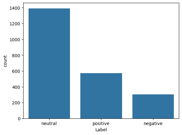
# Plot class distribution
import seaborn as sns
sns.countplot(x='Label', data=df)
<Axes: xlabel='Label', ylabel='count'>
32.4. Now install raw text tools#
from sklearn.model_selection import train_test_split
from sklearn.ensemble import RandomForestClassifier
from sklearn.metrics import accuracy_score
from sklearn.metrics import classification_report
from sklearn.metrics import roc_curve,auc
from sklearn.metrics import confusion_matrix
from sklearn.linear_model import LogisticRegression
from sklearn.model_selection import cross_val_score
# See Transformers from Hugging Face: https://huggingface.co/transformers/
# Simple Transformers: https://github.com/ThilinaRajapakse/simpletransformers

!pip install gensim
# !pip install transformers
Collecting gensim
  Downloading gensim-4.4.0-cp312-cp312-manylinux_2_24_x86_64.manylinux_2_28_x86_64.whl.metadata (8.4 kB)
Requirement already satisfied: numpy>=1.18.5 in /usr/local/lib/python3.12/dist-packages (from gensim) (2.0.2)
Requirement already satisfied: scipy>=1.7.0 in /usr/local/lib/python3.12/dist-packages (from gensim) (1.16.3)
Requirement already satisfied: smart_open>=1.8.1 in /usr/local/lib/python3.12/dist-packages (from gensim) (7.4.1)
Requirement already satisfied: wrapt in /usr/local/lib/python3.12/dist-packages (from smart_open>=1.8.1->gensim) (2.0.0)
Downloading gensim-4.4.0-cp312-cp312-manylinux_2_24_x86_64.manylinux_2_28_x86_64.whl (27.9 MB)
   ━━━━━━━━━━━━━━━━━━━━━━━━━━━━━━━━━━━━━━━━ 27.9/27.9 MB 44.2 MB/s eta 0:00:00
?25hInstalling collected packages: gensim
Successfully installed gensim-4.4.0
import json
from sklearn import feature_extraction, feature_selection, metrics
from sklearn import model_selection, naive_bayes, pipeline, manifold, preprocessing
import gensim
import gensim.downloader as gensim_api
from tensorflow.keras import models, layers, preprocessing as kprocessing
from tensorflow.keras import backend as K
from tensorflow.keras.utils import plot_model
import transformers
import nltk
nltk.download("stopwords")
nltk.download("wordnet")
nltk.download('omw-1.4')
stopwords = nltk.corpus.stopwords.words("english")
[nltk_data] Downloading package stopwords to /root/nltk_data...
[nltk_data]   Unzipping corpora/stopwords.zip.
[nltk_data] Downloading package wordnet to /root/nltk_data...
[nltk_data] Downloading package omw-1.4 to /root/nltk_data...
# Use texthero as an alternative text cleaner, instead of the code below
import re # regex

def removeNumbersStr(s):
    for c in range(10):
        n = str(c)
        s = s.replace(n," ")
    return s

def cleanText(text, stem=False, lemm=True, stop=True):
    text = re.sub(r'[^\w\s]', '', str(text).lower().strip())  # remove stuff
    text = removeNumbersStr(text)
    text = text.split()  # tokenize
    if stop is not None:  # remove stopwords
        text = [word for word in text if word not in stopwords]
    if stem == True:  # stemming
        ps = nltk.stem.porter.PorterStemmer()
        text = [ps.stem(word) for word in text]
    if lemm == True:
        lem = nltk.stem.wordnet.WordNetLemmatizer()
        text = [lem.lemmatize(word) for word in text]
    text = " ".join(text)
    return text
df["cleanTxt"] = [cleanText(df.Text[j]) for j in range(len(df.Label))]
print(df.shape)
df.head()
(2264, 3)
| Text | Label | cleanTxt | |
|---|---|---|---|
| 0 | According to Gran , the company has no plans t... | neutral | according gran company plan move production ru... |
| 1 | For the last quarter of 2010 , Componenta 's n... | positive | last quarter componenta net sale doubled eur e... |
| 2 | In the third quarter of 2010 , net sales incre... | positive | third quarter net sale increased eur mn operat... |
| 3 | Operating profit rose to EUR 13.1 mn from EUR ... | positive | operating profit rose eur mn eur mn correspond... |
| 4 | Operating profit totalled EUR 21.1 mn , up fro... | positive | operating profit totalled eur mn eur mn repres... |
df_train, df_test = model_selection.train_test_split(df, test_size=0.2)
y_train = df_train["Label"].values
y_test = df_test["Label"].values
# Choose BOW or TFIDF in NLTK
# vectorizer = feature_extraction.text.CountVectorizer(max_features=10000, ngram_range=(1,2))  # BOW
vectorizer = feature_extraction.text.TfidfVectorizer(max_features=10000, ngram_range=(1,2))  # TFIDF
corpus = df_train["cleanTxt"]
vectorizer.fit(corpus)
X_train = vectorizer.transform(corpus)
X_train
<Compressed Sparse Row sparse matrix of dtype 'float64'
	with 29553 stored elements and shape (1811, 10000)>
vocab = vectorizer.vocabulary_   # is a dict
list(vocab.keys())[:30]
['said',
 'board',
 'involve',
 'lot',
 'work',
 'people',
 'get',
 'paid',
 'time',
 'involve lot',
 'lot work',
 'work people',
 'get paid',
 'company',
 'generates',
 'net',
 'sale',
 'mln',
 'euro',
 'annually',
 'employ',
 'company generates',
 'generates net',
 'net sale',
 'sale mln',
 'mln euro',
 'euro mln',
 'mln annually',
 'reporting',
 'period']
X_train.shape
(1811, 10000)
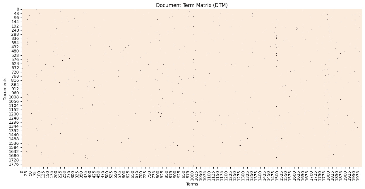
32.5. Visualize the DTM#
figure(figsize=(15,7))
sns.heatmap(X_train.todense() [:,np.random.randint(0,X_train.shape[1],2000)]==0,
            vmin=0, vmax=1, cbar=False).set_title('Document Term Matrix (DTM)')
xlabel('Terms'); ylabel('Documents')
Text(158.22222222222223, 0.5, 'Documents')
32.6. Reduce the dimension of the vocabulary#
# Feature reduction using feature selection in sklearn
# This can also be done using TextHero
y = df_train["Label"]
X_names = vectorizer.get_feature_names_out()
p_value_limit = 0.75
df_features = pd.DataFrame()
for cat in np.unique(y):
    chi2, p = feature_selection.chi2(X_train, y==cat)
    df_features = pd.concat([df_features, pd.DataFrame({"feature":X_names, "score":1-p, "y":cat})])
    df_features = df_features.sort_values(["y","score"],ascending=[True,False])
    df_features = df_features[df_features["score"]>p_value_limit]
X_names = df_features["feature"].unique().tolist()
print(type(X_names)); print(X_names[:10])
print("# features =",len(X_names))
<class 'list'>
['decreased', 'decreased eur', 'fell', 'eur mn', 'mn', 'operating loss', 'compared profit', 'sale decreased', 'eur', 'dropped']
# features = 1293
# !conda install -c conda-forge xgboost -y
32.7. TFIDF Transform Classification#
# Define Vectorizer
vectorizer = feature_extraction.text.TfidfVectorizer(vocabulary=X_names)
vectorizer.fit(corpus)
X_train = vectorizer.transform(corpus)
vocab = vectorizer.vocabulary_
print("Check vocab length:", len(vocab))

tmp = zeros(X_train.shape[0])
for j in range(len(tmp)):
    if y_train[j]=='negative':
        tmp[j] = 1
    elif y_train[j]=='positive':
        tmp[j] = 2
y_train = tmp

# Define Classifier
import xgboost as xgb
# classifier = xgb.XGBClassifier(objective="binary:logistic") # for 2 classes
classifier = xgb.XGBClassifier(objective="multi:softmax") # for multiclass
Check vocab length: 1293
# Pipeline using sklearn
model = pipeline.Pipeline([("vectorizer", vectorizer),
                           ("classifier", classifier)])
model["classifier"].fit(X_train, y_train)
X_test = df_test["cleanTxt"].values

# Accessing the classifier directly when making prediction
predicted = model["classifier"].predict(vectorizer.transform(X_test))  # Use transform here
predicted_prob = model["classifier"].predict_proba(vectorizer.transform(X_test))  # Use transform here
tmp = zeros(X_test.shape[0])
for j in range(len(tmp)):
    if y_test[j]=='negative':
        tmp[j] = 1
    elif y_test[j]=='positive':
        tmp[j] = 2
y_test = tmp

accuracy = metrics.accuracy_score(y_test, predicted)
# auc = metrics.roc_auc_score(y_test, predicted_prob[:,1])  # only for binary classification
print("Accuracy:", round(accuracy,2))
# print("Auc:", round(auc,2))
print("Detail:")
print(metrics.classification_report(y_test, predicted))
cm = metrics.confusion_matrix(y_test, predicted)
print(cm)
Accuracy: 0.85
Detail:
              precision    recall  f1-score   support

         0.0       0.89      0.96      0.92       271
         1.0       0.81      0.58      0.67        73
         2.0       0.75      0.75      0.75       109

    accuracy                           0.85       453
   macro avg       0.82      0.76      0.78       453
weighted avg       0.84      0.85      0.84       453

[[259   3   9]
 [ 13  42  18]
 [ 20   7  82]]
32.8. Using Embeddings#
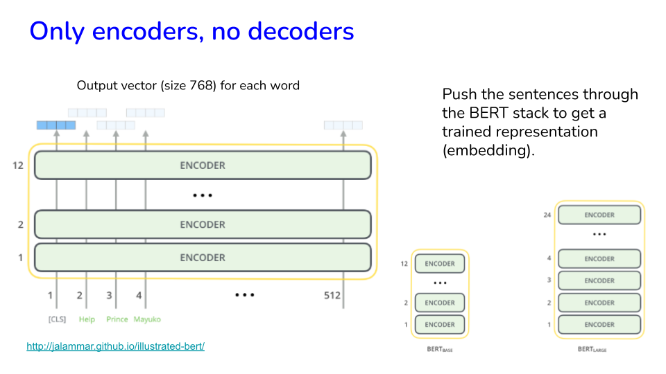
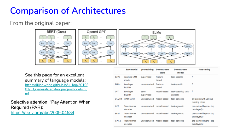
Ideally, we want an embedding model which gives us the smallest embedding vector and works great for the task. The smaller the embedding size, the lesser the compute required for training as well as inference.
Instead of TFIDF representations of text, we can use embeddings based on Word2Vec, Doc2Vec, etc. Much of these approaches have been superceded now by Transformer generated embeddings in the class of BERT models.
Slides: https://docs.google.com/presentation/d/1xhOocjNJ-6YU_jXPJb_Yi0Vloen65QCyM51S7-Dadfk/edit?usp=sharing
Image("NLP_images/BERT (0).png", width=900)
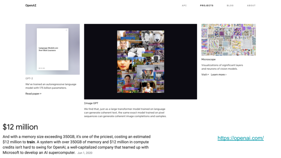
Image("NLP_images/BERT (1).png", width=900)
Image("NLP_images/models_timeline.png", width=900)
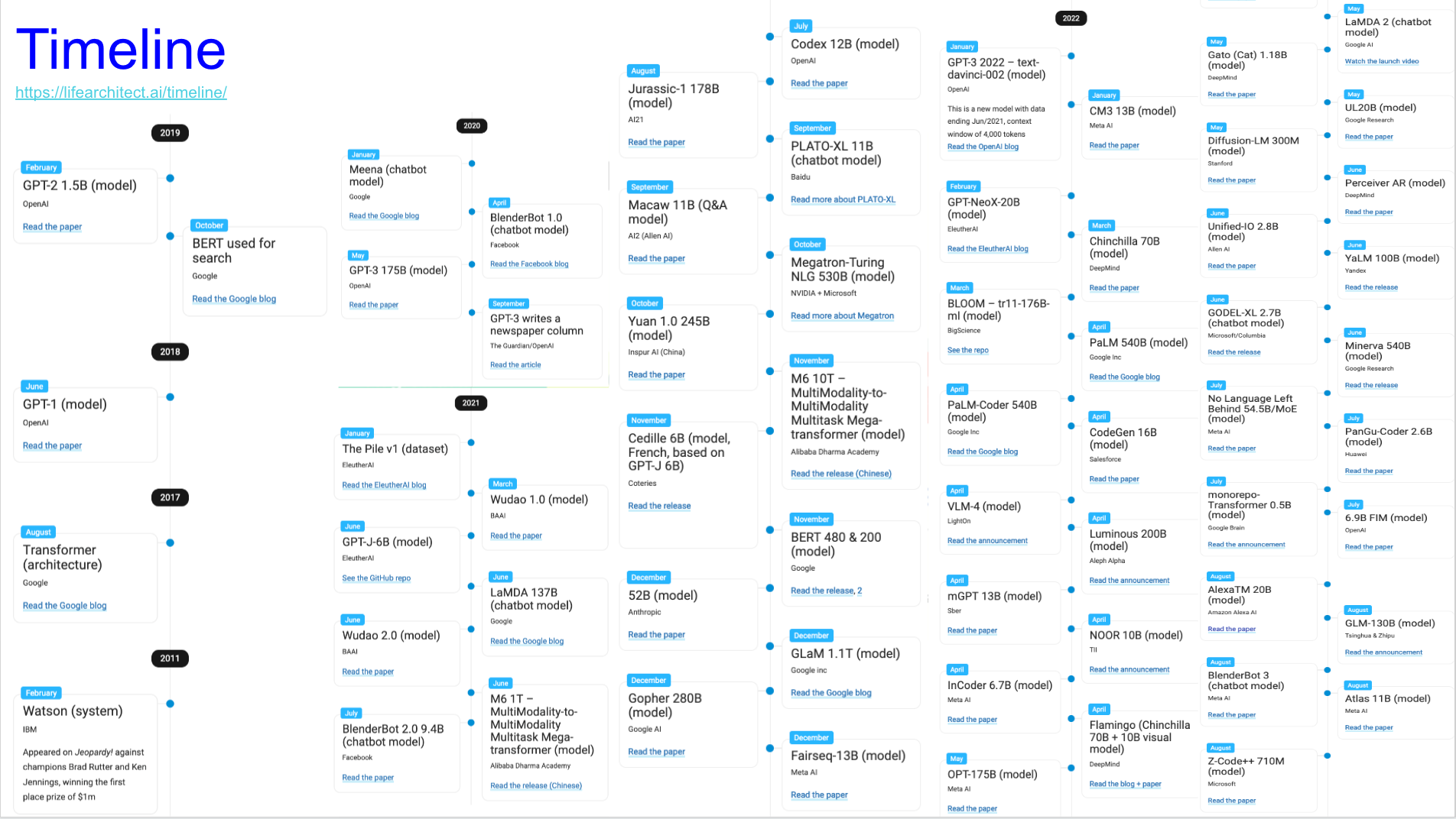
https://lifearchitect.ai/timeline/
Image("NLP_images/BERT (2).png", width=900)
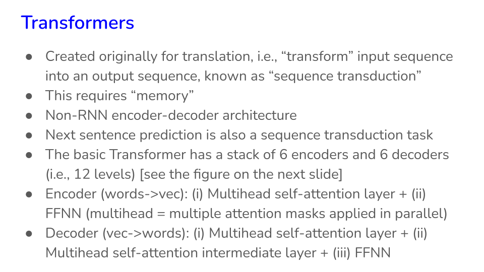
32.9. Transformers#
Read this amazing short book for a complete introduction to transformers.
Image("NLP_images/BERT (3).png", width=900)
Image("NLP_images/BERT (4).png", width=900)
Image("NLP_images/BERT (5).png", width=900)
Image("NLP_images/BERT (6).png", width=900)
Image("NLP_images/BERT (7).png", width=900)
# Image("NLP_images/BERT (8).png", width=900)
Image("NLP_images/BERT (11).png", width=900)
Image("NLP_images/BERT (10).png", width=900)
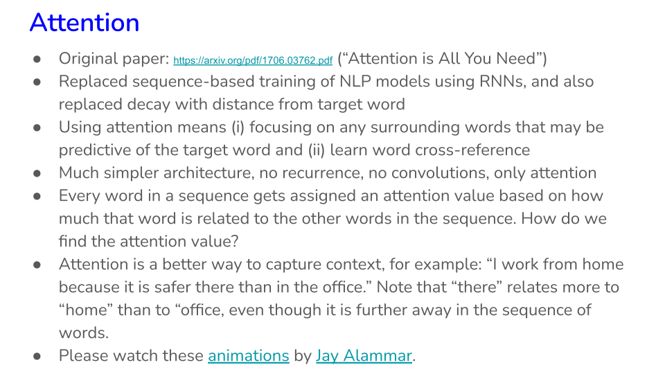
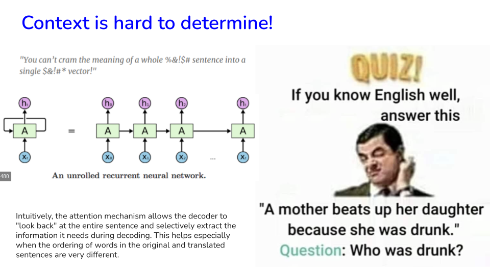
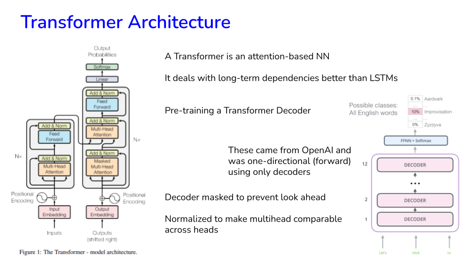
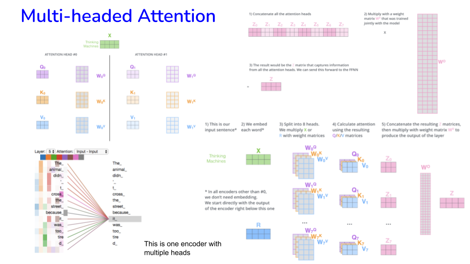
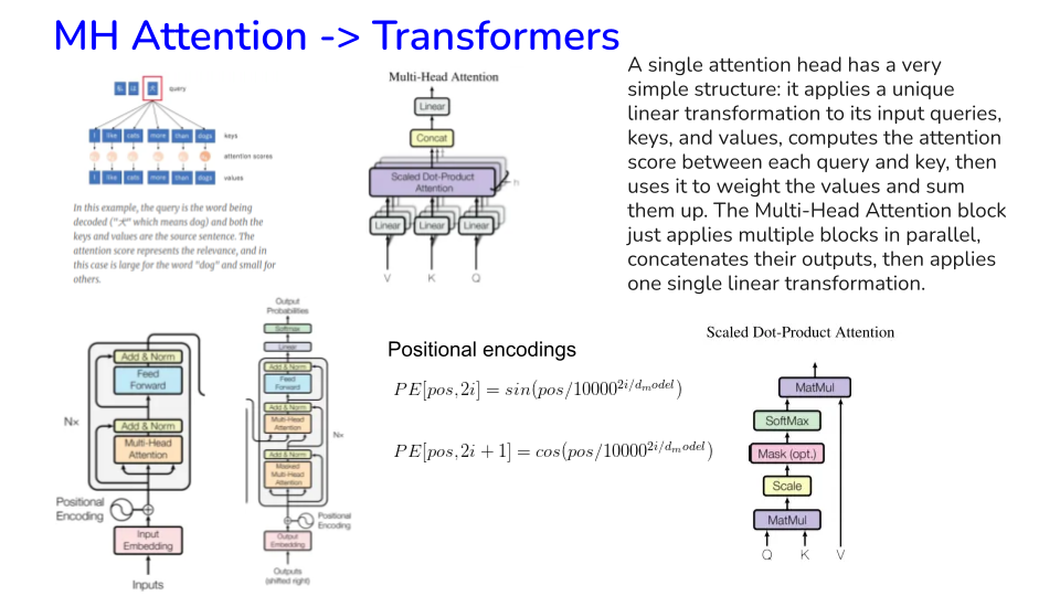
The main idea of Attention is to modify word vectors so that they have more context.
There is some controversy about when the term “attention” first entered the literature, going way back to the 1990s. For a full and very balanced discussion, see: https://www.turingpost.com/p/attention
Image("NLP_images/BERT (13).png", width=900)
Image("NLP_images/BERT (14).png", width=900)
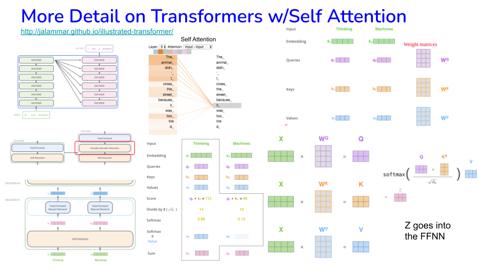
Ref: https://jalammar.github.io/illustrated-transformer
Image("NLP_images/BERT (15).png", width=900)
Image("NLP_images/BERT (16).png", width=900)
See the BertViz library for visualizing attention.
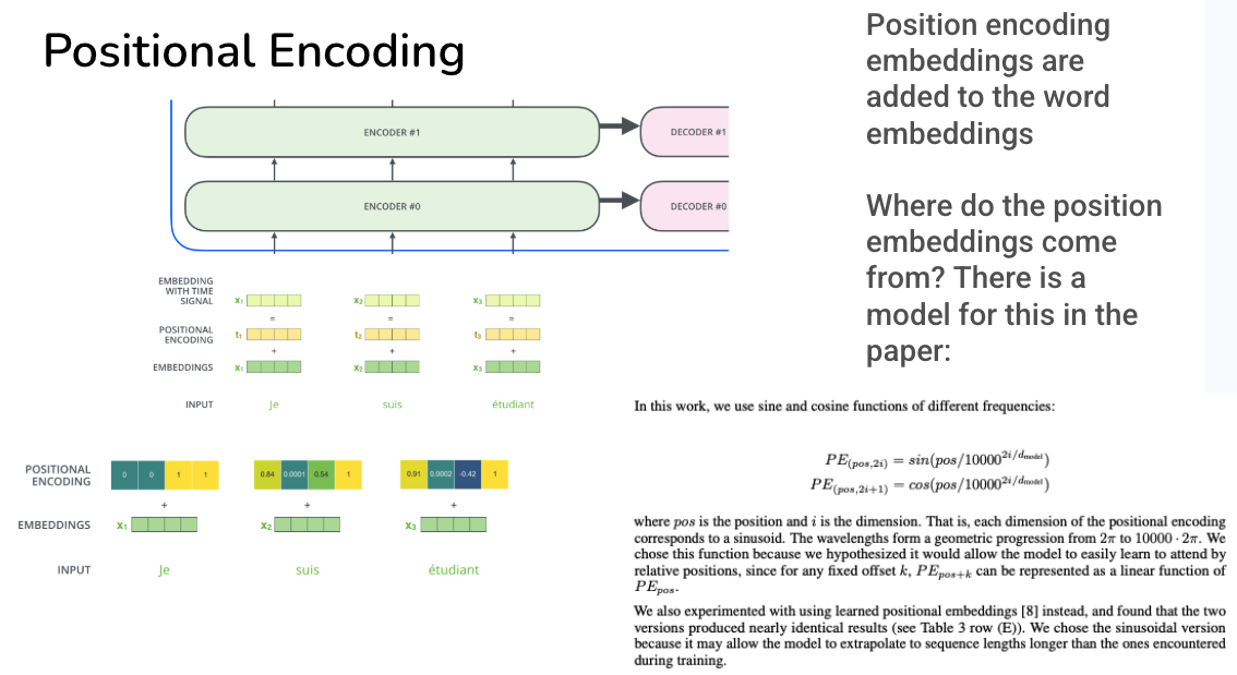
Image("NLP_images/Positional_encoding.png", width=900)
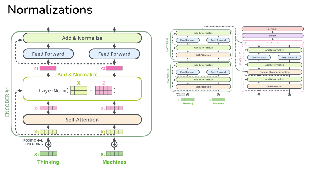
Image("NLP_images/Normalizations.png", width=900)
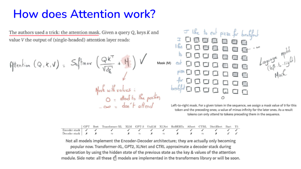
Image("NLP_images/BERT (12).png", width=900)
Image("NLP_images/BERT (17).png", width=900)
Image("NLP_images/BERT (9).png", width=900)
32.10. Transformers - Toy Example#
See also Layer Normalization: https://pytorch.org/docs/stable/generated/torch.nn.LayerNorm.html
# Code to exemplify transformers
# 2 tokens, embedding dimension of 4

# Embedding matrix
x = rand(2,4)
print(f"Input Embeddings:\n {x}")

# Set up weight matrices for query (Q), key (K), and value (V) vectors
wQ = rand(4,3)
wK = rand(4,3)
wV = rand(4,3)

# Generate the queries, keys, and value vectors
q = x.dot(wQ)
k = x.dot(wK)
v = x.dot(wV)

print(f"Query:\n {q}")
print(f"Key:\n {k}")
print(f"Value:\n {v}")

# Self attention for each word
score = q.dot(k.T)
print(f"Score:\n {score}") # each row is self attention for a word

# Divide by Sqrt of query dimension
sqrt_dk = sqrt(len(q[0]))
score = score/sqrt_dk
print(f"Sqrt dk: {sqrt_dk}\nRevised score:\n {score}")

# Softmax
softmax = np.exp(score) / np.sum(np.exp(score), axis=1, keepdims=True)
print(f"Softmax:\n {softmax}") # This gives the self-attention values

# z = Softmax x value
z = softmax.dot(v)
print(f"Z:\n {z}")

# Rescale back to original dimension using multiple heads (in this example we have just one head)
w0 = np.random.rand(3,4)
z = z.dot(w0)
print(f"Output:\n {z}") # Each row to be fed into the separate FFNNs to complete the encoder
Input Embeddings:
 [[0.71670422 0.32275089 0.46274821 0.95907814]
 [0.62480937 0.57130487 0.63743802 0.578689  ]]
Query:
 [[1.18875197 1.33293464 0.75381484]
 [1.18690097 1.43200107 0.94781579]]
Key:
 [[1.17981314 1.46183186 1.66963792]
 [1.11561407 1.32845185 1.40901822]]
Value:
 [[1.50858031 0.36449115 1.21013845]
 [1.31975521 0.47932063 1.2347729 ]]
Score:
 [[4.60962937 4.15906677]
 [5.07617534 4.56195762]]
Sqrt dk: 1.7320508075688772
Revised score:
 [[2.66137076 2.40123832]
 [2.9307312  2.63384746]]
Softmax:
 [[0.56466885 0.43533115]
 [0.57368054 0.42631946]]
Z:
 [[1.42637886 0.41448    1.22086259]
 [1.4280805  0.41344519 1.2206406 ]]
Output:
 [[1.67894233 1.56187961 2.60523998 2.15525082]
 [1.67945849 1.56272558 2.60564054 2.15486878]]
# Multiheads for Attention
# Suppose we have 6 of these Attention results and we put them side by side
# Then we get a matrix of size 2 x 24, lets create a dummy one here:
z = rand(2,24)

# We want to bring this down to a matrix of 2 x 4 in size
# Which means we need to multiply it by a matrix of dimension 24 x 4
wO = rand(24,4)
z = z.dot(wO)
print(f"Output:\n {z}") # Each row to be fed into the separate FFNNs to complete the encoder
Output:
 [[6.57705716 6.73567573 5.38936271 5.73943873]
 [5.85650206 5.50326831 4.16194226 4.85487406]]
Image("NLP_images/BERT (18).png", width=900)

Image("NLP_images/BERT (19).png", width=900)
Both schemes shown above are examples of “Self-supervised Learning”.
Image("NLP_images/BERT (20).png", width=900)
Image("NLP_images/BERT (21).png", width=900)
Image("NLP_images/BERT (22).png", width=900)
Image("NLP_images/BERT (23).png", width=900)
Image("NLP_images/BERT (24).png", width=900)
Image("NLP_images/BERT (25).png", width=900)
32.11. Recap of Transformers: https://drive.google.com/file/d/1LrzHTZoXP-PQ2Gzv1IOd4wJOfhtkKkzW/view?usp=sharing#
32.12. Transformers – Other Useful Links#
Video on transformers: https://www.youtube.com/watch?v=bCz4OMemCcA
3Blue1Brown: https://www.youtube.com/watch?v=wjZofJX0v4M (Transformers); https://www.youtube.com/watch?v=eMlx5fFNoYc (Attention)
Build a transformer from scratch: https://medium.com/towards-data-science/build-your-own-transformer-from-scratch-using-pytorch-84c850470dcb
Detailed view of transformers: https://e2eml.school/transformers.html
Understanding and coding attention: https://drive.google.com/file/d/1wzQ8q0gno23v8zoyP6_lCsa-DXg5xbqS/view?usp=sharing
Attnetion in Transformers: Concepts and Code in PyTorch (from DeepLearning.ai: https://learn.deeplearning.ai/courses/attention-in-transformers-concepts-and-code-in-pytorch/
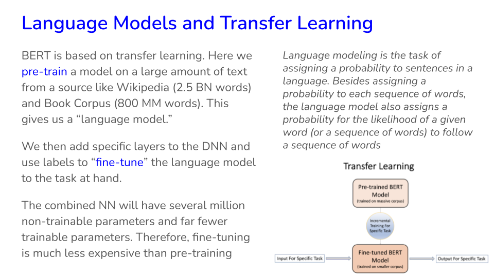
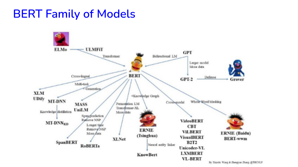
32.13. BERT (Summary)#
BERT piggybacks on Transformer models, for a technical overview, see: https://drive.google.com/file/d/1G4tEu0SQrYglVIvgRqY17Khlbhvuf-4s/view?usp=sharing
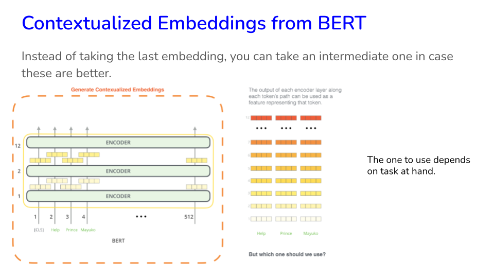
BERT handles context better than word embeddings. Therefore it takes care of polysemy, i.e., same word meaning different things in different context.
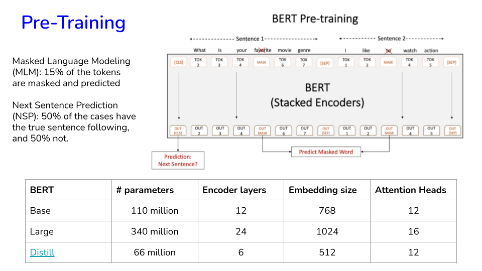
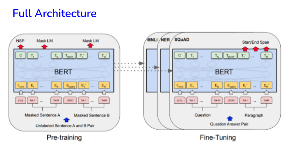
BERT is trained using a denoising objective (masked language modeling), where it aims to reconstruct a noisy version of a sentence back into its original version. The concept is similar to autoencoders.
The original BERT uses a next-sentence prediction objective, but it was shown in the RoBERTa paper that this training objective doesn’t help that much. In this way, BERT is trained on gigabytes of data from various sources (much of Wikipedia) in an unsupervised fashion.
Google Research and Toyota Technological Institute jointly released a much smaller/smarter Lite Bert called ALBERT. (“ALBERT: A Lite BERT for Self-supervised Learning of Language Representations”). BERT x-large has 1.27 Billion parameters, vs ALBERT x-large with 59 Million parameters! The core architecture of ALBERT is BERT-like in that it uses a transformer encoder architecture, along with GELU activation. It also uses the identical vocabulary size of 30K as used in the original BERT. (V=30,000).
The downside of BERT is compute: you definitely need a GPU.
Will Transformers take over everything in NLP and computer vision? https://www.quantamagazine.org/will-transformers-take-over-artificial-intelligence-20220310/
32.14. BERT with transfer learning#
BERT input has a special structure. Take the sequence of words - “The paycheck protection program” and it gets encoded as
CLS | The | paycheck | protection | program | SEP | PAD | PAD | PAD
There are 3 vectors that are generated by this:
(1) Token IDs: these are integers that refer to the vocab index. Some have fixed IDs such as
CLS = 101 (start id)
UNK = 100 (unknown id)
SEP = 102 (end/separator id)
PAD = 0 (padding slots id)
The actual words get their ids from the vocab.
(2) Mask = 1 from CLS through SEP, 0 thereafter. It delineates the text from its padding.
(3) Segment = 1 for SEP, zero elsewhere. It delineates sentences.
Steps:
tokenize + transform + create embedding
See the first element of the embedding that is generated, it is what is passed to the NN.
import transformers
# Just trying out original BERT
txt = "love the show"
tokenizer = transformers.BertTokenizer.from_pretrained('bert-base-uncased', do_lower_case=True)
input_ids = array(tokenizer.encode(txt))[None,:]

## Use language model to return hidden layer with embeddings
# Changed TFBertModel to TFAutoModel and added from_pt=True
nlp = transformers.TFAutoModel.from_pretrained('bert-base-uncased', from_pt=True)
embedding = nlp(input_ids)
/usr/local/lib/python3.12/dist-packages/huggingface_hub/utils/_auth.py:94: UserWarning:
The secret `HF_TOKEN` does not exist in your Colab secrets.
To authenticate with the Hugging Face Hub, create a token in your settings tab (https://huggingface.co/settings/tokens), set it as secret in your Google Colab and restart your session.
You will be able to reuse this secret in all of your notebooks.
Please note that authentication is recommended but still optional to access public models or datasets.
  warnings.warn(
TensorFlow and JAX classes are deprecated and will be removed in Transformers v5. We recommend migrating to PyTorch classes or pinning your version of Transformers.
Some weights of the PyTorch model were not used when initializing the TF 2.0 model TFBertModel: ['cls.predictions.transform.LayerNorm.weight', 'cls.predictions.transform.dense.weight', 'cls.predictions.bias', 'cls.predictions.decoder.weight', 'cls.predictions.transform.dense.bias', 'cls.seq_relationship.weight', 'cls.seq_relationship.bias', 'cls.predictions.transform.LayerNorm.bias']
- This IS expected if you are initializing TFBertModel from a PyTorch model trained on another task or with another architecture (e.g. initializing a TFBertForSequenceClassification model from a BertForPreTraining model).
- This IS NOT expected if you are initializing TFBertModel from a PyTorch model that you expect to be exactly identical (e.g. initializing a TFBertForSequenceClassification model from a BertForSequenceClassification model).
All the weights of TFBertModel were initialized from the PyTorch model.
If your task is similar to the task the model of the checkpoint was trained on, you can already use TFBertModel for predictions without further training.
print("Structure of BERT input (size of text + 2):", input_ids)
print("Length of embedding structure:", len(embedding))
print("Shape of first element of embedding:", embedding[0][0].shape)  # size of input ids, BERT input vector size
print("Shape of second element of embedding:", embedding[1][0].shape)  #
Structure of BERT input (size of text + 2): [[ 101 2293 1996 2265  102]]
Length of embedding structure: 2
Shape of first element of embedding: (5, 768)
Shape of second element of embedding: (768,)
32.15. Use distill BERT from Hugging Face#
https://huggingface.co/docs/transformers/index
tokenizer = transformers.AutoTokenizer.from_pretrained('distilbert-base-uncased')

## Use language model to return hidden layer with embeddings
# Use TFDistilBertModel for DistilBERT
nlp = transformers.TFAutoModel.from_pretrained('distilbert-base-uncased', from_pt=True)
embedding = nlp(input_ids)
Some weights of the PyTorch model were not used when initializing the TF 2.0 model TFDistilBertModel: ['vocab_projector.weight', 'vocab_transform.weight', 'vocab_layer_norm.bias', 'vocab_projector.bias', 'vocab_layer_norm.weight', 'vocab_transform.bias']
- This IS expected if you are initializing TFDistilBertModel from a PyTorch model trained on another task or with another architecture (e.g. initializing a TFBertForSequenceClassification model from a BertForPreTraining model).
- This IS NOT expected if you are initializing TFDistilBertModel from a PyTorch model that you expect to be exactly identical (e.g. initializing a TFBertForSequenceClassification model from a BertForSequenceClassification model).
All the weights of TFDistilBertModel were initialized from the PyTorch model.
If your task is similar to the task the model of the checkpoint was trained on, you can already use TFDistilBertModel for predictions without further training.
print("Structure of BERT input (size of text + 2):", input_ids)
print("Embedding:", embedding)
print("Embedding:", embedding[0])
Structure of BERT input (size of text + 2): [[ 101 2293 1996 2265  102]]
Embedding: TFBaseModelOutput(last_hidden_state=<tf.Tensor: shape=(1, 5, 768), dtype=float32, numpy=
array([[[-0.04657122, -0.13871671,  0.13348138, ..., -0.1272782 ,
          0.17813185,  0.24944863],
        [ 1.1028556 ,  0.26482472,  0.6136154 , ..., -0.33415368,
          0.8009101 ,  0.11689214],
        [-0.16672158, -1.0389844 ,  0.2690747 , ..., -0.0717033 ,
          0.6851587 , -0.24214913],
        [ 0.08075567, -0.7811562 ,  0.43119788, ...,  0.17319538,
          0.45068687, -0.5403498 ],
        [ 0.94134337,  0.20700857, -0.30040848, ...,  0.19120099,
         -0.58041805, -0.1728739 ]]], dtype=float32)>, hidden_states=None, attentions=None)
Embedding: tf.Tensor(
[[[-0.04657122 -0.13871671  0.13348138 ... -0.1272782   0.17813185
    0.24944863]
  [ 1.1028556   0.26482472  0.6136154  ... -0.33415368  0.8009101
    0.11689214]
  [-0.16672158 -1.0389844   0.2690747  ... -0.0717033   0.6851587
   -0.24214913]
  [ 0.08075567 -0.7811562   0.43119788 ...  0.17319538  0.45068687
   -0.5403498 ]
  [ 0.94134337  0.20700857 -0.30040848 ...  0.19120099 -0.58041805
   -0.1728739 ]]], shape=(1, 5, 768), dtype=float32)
# Reuse the data from the TFIDF classification problem
corpus = df_train["Text"] # use Text not cleanTxt as we want context and need to keep the sentences as they are
len(corpus)
1811
## Prepare BERT input for the training dataset
max_seq_length = 160  # The longest sentences in the dataset are less than this, adjust as needed

# Create a string of BERT and word tokens
corpus_tokenized = ["[CLS] "+" ".join(tokenizer.tokenize(re.sub(r'[^\w\s]+|\n', '',
                    str(txt).lower().strip()))[:max_seq_length])+" [SEP] " for txt in corpus]

## 1. Generate index values for the tokens and add padding, then make sure tokens are at max sequence length
txt2seq = [txt + " [PAD]"*(10+max_seq_length-len(txt.split(" "))) for txt in corpus_tokenized] # added 10 for extra padding (hack)
idx = [tokenizer.encode(seq)[1:-1][:max_seq_length] for seq in txt2seq]  # Need to drop the first and last element, and set no of token to max_seq_len

## 2. Generate masks
masks = [[1]*len(txt.split(" ")) + [0]*(max_seq_length - len( txt.split(" "))) for txt in corpus_tokenized]

## 3. Generate segments
segments = []
for seq in txt2seq:
    temp, i = [], 0
    for token in seq.split(" "):
        temp.append(i)
        if token == "[SEP]":
            i += 1
    segments.append(temp)

# Finally, put all 3 elements into a feature matrix
X_train = [asarray(idx, dtype='int32'),
           asarray(masks, dtype='int32'),
           asarray(segments, dtype='int32')]
# X_train is a 3 dimension tensor
print(len(X_train))  # one each for Token ID, Mask, Segment arrays
print(len(X_train[0])) # Size of the training set
print(len(X_train[0][0])) # max sequence length + 2 (for CLS and SEP)
3
1811
160
df_train
| Text | Label | cleanTxt | |
|---|---|---|---|
| 1030 | Sullivan said some of the boards `` really inv... | neutral | sullivan said board really involve lot work pe... |
| 284 | The company generates net sales of about 600 m... | neutral | company generates net sale mln euro mln annual... |
| 781 | After the reporting period , BioTie North Amer... | positive | reporting period biotie north american licensi... |
| 1935 | The purchase price will be paid in cash upon t... | neutral | purchase price paid cash upon closure transact... |
| 2102 | In Finland , the Bank of +àland reports its op... | negative | finland bank àland report operating profit fel... |
| ... | ... | ... | ... |
| 2117 | Finnish GeoSentric 's net sales decreased to E... | negative | finnish geosentric net sale decreased eur janu... |
| 1798 | The ongoing project where Tekla Structures is ... | neutral | ongoing project tekla structure used vashi exh... |
| 1800 | The order also covers design services , hardwa... | neutral | order also cover design service hardware softw... |
| 913 | 128,538 shares can still be subscribed for wit... | neutral | share still subscribed series e share option max |
| 1892 | The company reported today an operating loss o... | negative | company reported today operating loss eur net ... |
1811 rows × 3 columns
k = randint(len(X_train[0])) # Pick a random sentence, try 302
# print(df_train["Text"][k])
print(len(X_train[0][k]))
print(X_train[0][k])   # Token ids
print(X_train[1][k])   # mask
print(X_train[2][k])   # segment
160
[  101  1996  2194  2036  2805 26947  1001  1001  1042 21701  2132  1997
  1996  2569  5127  3131  2029  2950  1996 24209  1001  1001  2396  1001
  1001  1051  5127  3197  1999  2139  1001  1001 16216  2099  1001  1001
  2005  1001  1001  1055  4701  1998  2047  3317  3915  1996  3131  1999
  2097  1001  1001 22564  2762  2004  2092  2004  2811  1001  1001  5127
  1998  3653  1001  1001  6904  1001  1001  1038  1999 13642  1001  1001
  2358  2050  1998  5127  2326  2803 13649  1999  2139  1001  1001 16216
  2099  1001  1001  2005  1001  1001  1055   102     0     0     0     0
     0     0     0     0     0     0     0     0     0     0     0     0
     0     0     0     0     0     0     0     0     0     0     0     0
     0     0     0     0     0     0     0     0     0     0     0     0
     0     0     0     0     0     0     0     0     0     0     0     0
     0     0     0     0     0     0     0     0     0     0     0     0
     0     0     0     0]
[1 1 1 1 1 1 1 1 1 1 1 1 1 1 1 1 1 1 1 1 1 1 1 1 1 1 1 1 1 1 1 1 1 1 1 1 1
 1 1 1 1 1 1 1 1 1 1 1 1 1 1 1 1 1 1 1 1 1 1 1 1 1 0 0 0 0 0 0 0 0 0 0 0 0
 0 0 0 0 0 0 0 0 0 0 0 0 0 0 0 0 0 0 0 0 0 0 0 0 0 0 0 0 0 0 0 0 0 0 0 0 0
 0 0 0 0 0 0 0 0 0 0 0 0 0 0 0 0 0 0 0 0 0 0 0 0 0 0 0 0 0 0 0 0 0 0 0 0 0
 0 0 0 0 0 0 0 0 0 0 0 0]
[0 0 0 0 0 0 0 0 0 0 0 0 0 0 0 0 0 0 0 0 0 0 0 0 0 0 0 0 0 0 0 0 0 0 0 0 0
 0 0 0 0 0 0 0 0 0 0 0 0 0 0 0 0 0 0 0 0 0 0 0 0 1 1 1 1 1 1 1 1 1 1 1 1 1
 1 1 1 1 1 1 1 1 1 1 1 1 1 1 1 1 1 1 1 1 1 1 1 1 1 1 1 1 1 1 1 1 1 1 1 1 1
 1 1 1 1 1 1 1 1 1 1 1 1 1 1 1 1 1 1 1 1 1 1 1 1 1 1 1 1 1 1 1 1 1 1 1 1 1
 1 1 1 1 1 1 1 1 1 1 1 1 1 1 1 1 1 1 1 1 1 1]
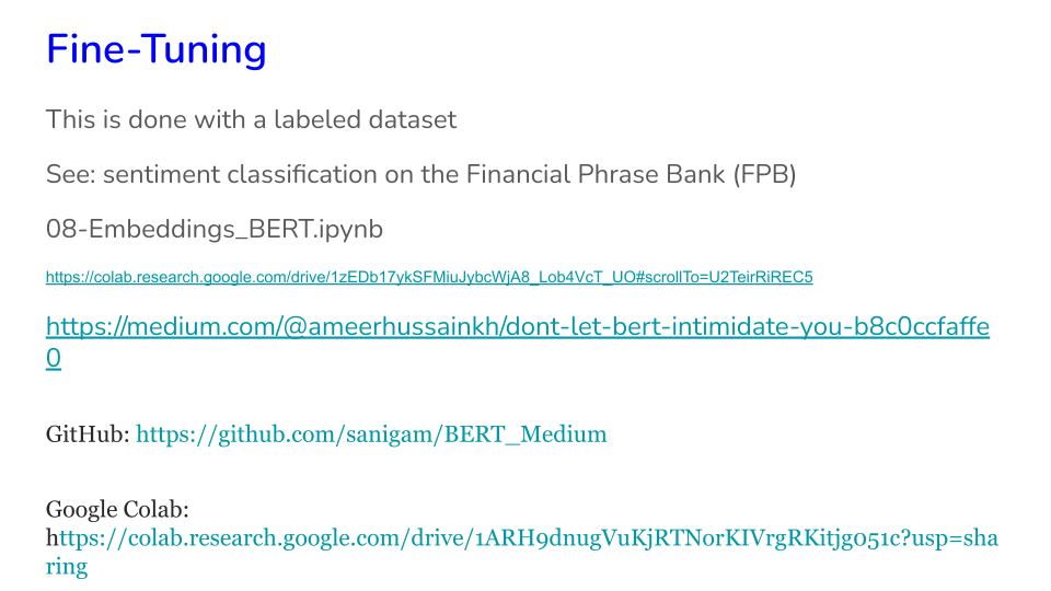
32.16. Fine-Tuning#
We are using DistilBERT below, which only requires the token IDs and masks (not segments).
# Build up model
import tensorflow as tf
from tensorflow import keras
from tensorflow.keras import layers, models
import transformers
import numpy as np

## inputs
idx = layers.Input((max_seq_length,), dtype="int32", name="input_idx")
masks = layers.Input((max_seq_length,), dtype="int32", name="input_masks")
segments = layers.Input((max_seq_length,), dtype="int32", name="input_segments")
## pre-trained bert with config
config = transformers.DistilBertConfig(dropout=0.2, attention_dropout=0.2)
config.output_hidden_states = False
nlp = transformers.TFAutoModel.from_pretrained('distilbert-base-uncased', config=config, from_pt=True)

# Wrap the DistilBERT call in a Lambda layer and specify output_shape
bert_out = layers.Lambda(
    lambda x: nlp(x[0], attention_mask=x[1])[0],
    output_shape=(max_seq_length, nlp.config.hidden_size)  # Add output_shape
)([idx, masks])

## fine-tuning
x = layers.GlobalAveragePooling1D()(bert_out)
x = layers.Dense(64, activation="relu")(x)
y_out = layers.Dense(len(np.unique(y_train)),activation='softmax')(x)
## compile
model = models.Model([idx, masks], y_out)
for layer in model.layers[:3]:
    layer.trainable = False

model.compile(loss='sparse_categorical_crossentropy', optimizer='adam', metrics=['accuracy'])
model.summary()
Some weights of the PyTorch model were not used when initializing the TF 2.0 model TFDistilBertModel: ['vocab_projector.weight', 'vocab_transform.weight', 'vocab_layer_norm.bias', 'vocab_projector.bias', 'vocab_layer_norm.weight', 'vocab_transform.bias']
- This IS expected if you are initializing TFDistilBertModel from a PyTorch model trained on another task or with another architecture (e.g. initializing a TFBertForSequenceClassification model from a BertForPreTraining model).
- This IS NOT expected if you are initializing TFDistilBertModel from a PyTorch model that you expect to be exactly identical (e.g. initializing a TFBertForSequenceClassification model from a BertForSequenceClassification model).
All the weights of TFDistilBertModel were initialized from the PyTorch model.
If your task is similar to the task the model of the checkpoint was trained on, you can already use TFDistilBertModel for predictions without further training.
Model: "functional_1"
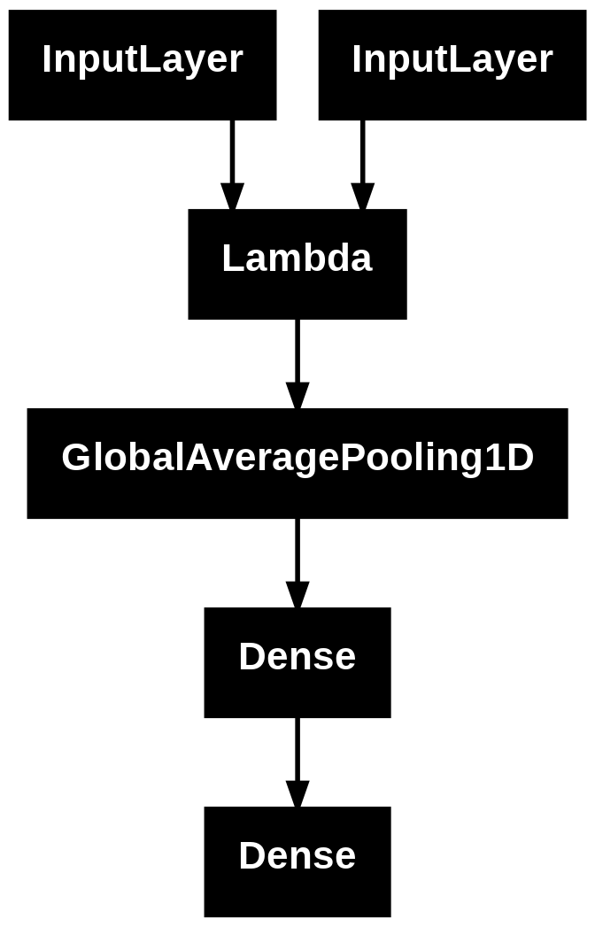
┏━━━━━━━━━━━━━━━━━━━━━┳━━━━━━━━━━━━━━━━━━━┳━━━━━━━━━━━━┳━━━━━━━━━━━━━━━━━━━┓
┃ Layer (type)        ┃ Output Shape      ┃    Param # ┃ Connected to      ┃
┡━━━━━━━━━━━━━━━━━━━━━╇━━━━━━━━━━━━━━━━━━━╇━━━━━━━━━━━━╇━━━━━━━━━━━━━━━━━━━┩
│ input_idx           │ (None, 160)       │          0 │ -                 │
│ (InputLayer)        │                   │            │                   │
├─────────────────────┼───────────────────┼────────────┼───────────────────┤
│ input_masks         │ (None, 160)       │          0 │ -                 │
│ (InputLayer)        │                   │            │                   │
├─────────────────────┼───────────────────┼────────────┼───────────────────┤
│ lambda_1 (Lambda)   │ (None, 160, 768)  │          0 │ input_idx[0][0],  │
│                     │                   │            │ input_masks[0][0] │
├─────────────────────┼───────────────────┼────────────┼───────────────────┤
│ global_average_poo… │ (None, 768)       │          0 │ lambda_1[0][0]    │
│ (GlobalAveragePool… │                   │            │                   │
├─────────────────────┼───────────────────┼────────────┼───────────────────┤
│ dense_2 (Dense)     │ (None, 64)        │     49,216 │ global_average_p… │
├─────────────────────┼───────────────────┼────────────┼───────────────────┤
│ dense_3 (Dense)     │ (None, 3)         │        195 │ dense_2[0][0]     │
└─────────────────────┴───────────────────┴────────────┴───────────────────┘
Total params: 49,411 (193.01 KB)
Trainable params: 49,411 (193.01 KB)
Non-trainable params: 0 (0.00 B)
plot_model(model) # option to_file=
# Create label y
dic_y_mapping = {0:'neutral', 1:'negative', 2:'positive'}
# Create inverse_dic mapping string labels to numerical labels
inverse_dic = {'neutral': 0, 'negative': 1, 'positive': 2}
print(len(X_train[1]))
print(unique(y_train))
1811
[0. 1. 2.]
%%time
## train
# Convert y_train to numerical labels just before training
y_train_numerical = np.array([inverse_dic[y] for y in df_train["Label"].values])
training = model.fit(x=X_train[:2], y=y_train_numerical, batch_size=32, epochs=10, shuffle=True, verbose=1, validation_split=0.3)
Epoch 1/10
40/40 ━━━━━━━━━━━━━━━━━━━━ 23s 330ms/step - accuracy: 0.5850 - loss: 0.8931 - val_accuracy: 0.7702 - val_loss: 0.5590
Epoch 2/10
40/40 ━━━━━━━━━━━━━━━━━━━━ 7s 178ms/step - accuracy: 0.7570 - loss: 0.5566 - val_accuracy: 0.7831 - val_loss: 0.4982
Epoch 3/10
40/40 ━━━━━━━━━━━━━━━━━━━━ 7s 179ms/step - accuracy: 0.7850 - loss: 0.4885 - val_accuracy: 0.8364 - val_loss: 0.4197
Epoch 4/10
40/40 ━━━━━━━━━━━━━━━━━━━━ 7s 182ms/step - accuracy: 0.8473 - loss: 0.3879 - val_accuracy: 0.8327 - val_loss: 0.4295
Epoch 5/10
40/40 ━━━━━━━━━━━━━━━━━━━━ 7s 183ms/step - accuracy: 0.8439 - loss: 0.3855 - val_accuracy: 0.8529 - val_loss: 0.3704
Epoch 6/10
40/40 ━━━━━━━━━━━━━━━━━━━━ 7s 186ms/step - accuracy: 0.8590 - loss: 0.3527 - val_accuracy: 0.8511 - val_loss: 0.3633
Epoch 7/10
40/40 ━━━━━━━━━━━━━━━━━━━━ 7s 184ms/step - accuracy: 0.8893 - loss: 0.3118 - val_accuracy: 0.8493 - val_loss: 0.3623
Epoch 8/10
40/40 ━━━━━━━━━━━━━━━━━━━━ 7s 186ms/step - accuracy: 0.8782 - loss: 0.3017 - val_accuracy: 0.8585 - val_loss: 0.3579
Epoch 9/10
40/40 ━━━━━━━━━━━━━━━━━━━━ 7s 187ms/step - accuracy: 0.8748 - loss: 0.3115 - val_accuracy: 0.8364 - val_loss: 0.3569
Epoch 10/10
40/40 ━━━━━━━━━━━━━━━━━━━━ 7s 188ms/step - accuracy: 0.8854 - loss: 0.2980 - val_accuracy: 0.8676 - val_loss: 0.3510
CPU times: user 23.2 s, sys: 2.64 s, total: 25.9 s
Wall time: 1min 28s
# train labels
predicted_prob = model.predict(X_train[:2])
dic_y_mapping = {0:'neutral', 1:'negative', 2:'positive'}  # for the financial phrase bank dataset
predicted = [dic_y_mapping[argmax(pred)] for pred in predicted_prob]
57/57 ━━━━━━━━━━━━━━━━━━━━ 12s 178ms/step
# Convert y_train to numerical labels, similar to how predicted was transformed
tmp = zeros(len(y_train))
for j in range(len(tmp)):
    if y_train[j]=='negative':
        tmp[j] = 1
    elif y_train[j]=='positive':
        tmp[j] = 2
y_test = tmp

# Convert predicted labels from strings to numerical labels
predicted_numerical = [inverse_dic[pred] for pred in predicted]

accuracy = metrics.accuracy_score(y_train, predicted_numerical)
# auc = metrics.roc_auc_score(y_test, predicted_prob[:,1])  # only for binary classification
print("Accuracy:", round(accuracy,2))
# print("Auc:", round(auc,2))
print("Detail:")
print(metrics.classification_report(y_train, predicted_numerical))
cm = metrics.confusion_matrix(y_train, predicted_numerical)
print(cm)
Accuracy: 0.89
Detail:
              precision    recall  f1-score   support

         0.0       0.95      0.95      0.95      1120
         1.0       0.69      0.92      0.79       230
         2.0       0.88      0.73      0.80       461

    accuracy                           0.89      1811
   macro avg       0.84      0.87      0.85      1811
weighted avg       0.90      0.89      0.89      1811

[[1066   19   35]
 [   8  211   11]
 [  48   75  338]]
TFIDF accuracy = 80-85%
Word2Vec accuracy = 70-75%
BERT accuracy = 82-89%
32.17. REFERENCES#
Using BERT for the first time (by J Alammar): http://jalammar.github.io/a-visual-guide-to-using-bert-for-the-first-time/; code: https://colab.research.google.com/github/jalammar/jalammar.github.io/blob/master/notebooks/bert/A_Visual_Notebook_to_Using_BERT_for_the_First_Time.ipynb
Stanford Sentiment Treebank: https://nlp.stanford.edu/sentiment/index.html
32.18. From the reference above, using the SST dataset (movie reviews)#
from sklearn.linear_model import LogisticRegression
from sklearn.model_selection import GridSearchCV
from sklearn.model_selection import cross_val_score
import torch
import transformers as ppb
import warnings
warnings.filterwarnings('ignore')
df_large = pd.read_csv('https://github.com/clairett/pytorch-sentiment-classification/raw/master/data/SST2/train.tsv', delimiter='\t', header=None)
print(df_large.shape)
df_large.head()
(6920, 2)
| 0 | 1 | |
|---|---|---|
| 0 | a stirring , funny and finally transporting re... | 1 |
| 1 | apparently reassembled from the cutting room f... | 0 |
| 2 | they presume their audience wo n't sit still f... | 0 |
| 3 | this is a visually stunning rumination on love... | 1 |
| 4 | jonathan parker 's bartleby should have been t... | 1 |
# Is the dataset balanced in labels?
df = df_large[:1500]  # take a small subset
df[1].value_counts()
| count | |
|---|---|
| 1 | |
| 1 | 782 |
| 0 | 718 |
32.19. Get the pre-trained model#
# For DistilBERT:
model_class, tokenizer_class, pretrained_weights = (ppb.DistilBertModel, ppb.DistilBertTokenizer, 'distilbert-base-uncased')

## Want BERT instead of distilBERT? Uncomment the following line:
#model_class, tokenizer_class, pretrained_weights = (ppb.BertModel, ppb.BertTokenizer, 'bert-base-uncased')

# Load pretrained model/tokenizer
tokenizer = tokenizer_class.from_pretrained(pretrained_weights)
model = model_class.from_pretrained(pretrained_weights)
# Get tokenized version
tokenized = df[0].apply((lambda x: tokenizer.encode(x, add_special_tokens=True)))
print(tokenized.shape)
tokenized[0]
(1500,)
[101,
 1037,
 18385,
 1010,
 6057,
 1998,
 2633,
 18276,
 2128,
 16603,
 1997,
 5053,
 1998,
 1996,
 6841,
 1998,
 5687,
 5469,
 3152,
 102]
32.20. Construct token IDs and masks#
# Add padding and set max len to the longest entry in the dataset
max_len = 0
for i in tokenized.values:
    if len(i) > max_len:
        max_len = len(i)

padded = array([i + [0]*(max_len-len(i)) for i in tokenized.values])
print(array(padded).shape)
padded[:3]
(1500, 59)
array([[  101,  1037, 18385,  1010,  6057,  1998,  2633, 18276,  2128,
        16603,  1997,  5053,  1998,  1996,  6841,  1998,  5687,  5469,
         3152,   102,     0,     0,     0,     0,     0,     0,     0,
            0,     0,     0,     0,     0,     0,     0,     0,     0,
            0,     0,     0,     0,     0,     0,     0,     0,     0,
            0,     0,     0,     0,     0,     0,     0,     0,     0,
            0,     0,     0,     0,     0],
       [  101,  4593,  2128, 27241, 23931,  2013,  1996,  6276,  2282,
         2723,  1997,  2151,  2445, 12217,  7815,   102,     0,     0,
            0,     0,     0,     0,     0,     0,     0,     0,     0,
            0,     0,     0,     0,     0,     0,     0,     0,     0,
            0,     0,     0,     0,     0,     0,     0,     0,     0,
            0,     0,     0,     0,     0,     0,     0,     0,     0,
            0,     0,     0,     0,     0],
       [  101,  2027,  3653, 23545,  2037,  4378, 24185,  1050,  1005,
         1056,  4133,  2145,  2005,  1037, 11507, 10800,  1010,  2174,
        14036,  2135,  3591,  1010,  2061,  2027, 19817,  4140,  2041,
         1996,  7511,  2671,  4349,  3787,  1997, 11829,  7168,  9219,
         1998, 28971,  2308,  1999,  8301,  8737,  2100,  4253,   102,
            0,     0,     0,     0,     0,     0,     0,     0,     0,
            0,     0,     0,     0,     0]])
# Add a mask to let BERT know where the real tokens are and not the padding
# Essentially we can use zero for the padding mask so those tokens do not compute
attention_mask = where(padded != 0, 1, 0)
print(attention_mask.shape)
attention_mask[:3]
(1500, 59)
array([[1, 1, 1, 1, 1, 1, 1, 1, 1, 1, 1, 1, 1, 1, 1, 1, 1, 1, 1, 1, 0, 0,
        0, 0, 0, 0, 0, 0, 0, 0, 0, 0, 0, 0, 0, 0, 0, 0, 0, 0, 0, 0, 0, 0,
        0, 0, 0, 0, 0, 0, 0, 0, 0, 0, 0, 0, 0, 0, 0],
       [1, 1, 1, 1, 1, 1, 1, 1, 1, 1, 1, 1, 1, 1, 1, 1, 0, 0, 0, 0, 0, 0,
        0, 0, 0, 0, 0, 0, 0, 0, 0, 0, 0, 0, 0, 0, 0, 0, 0, 0, 0, 0, 0, 0,
        0, 0, 0, 0, 0, 0, 0, 0, 0, 0, 0, 0, 0, 0, 0],
       [1, 1, 1, 1, 1, 1, 1, 1, 1, 1, 1, 1, 1, 1, 1, 1, 1, 1, 1, 1, 1, 1,
        1, 1, 1, 1, 1, 1, 1, 1, 1, 1, 1, 1, 1, 1, 1, 1, 1, 1, 1, 1, 1, 1,
        1, 0, 0, 0, 0, 0, 0, 0, 0, 0, 0, 0, 0, 0, 0]])
32.21. Run token IDs and attention masks through BERT to get embeddings#
%%time
input_ids = torch.tensor(padded)
attention_mask = torch.tensor(attention_mask)

with torch.no_grad():
    last_hidden_states = model(input_ids, attention_mask=attention_mask)  #embeddings
CPU times: user 2min 3s, sys: 15.1 s, total: 2min 18s
Wall time: 2min 47s
# Embeddings from BERT
print(len(last_hidden_states[0][:,0,:]))
last_hidden_states[0][:,0,:]
1500
tensor([[-0.2159, -0.1403,  0.0083,  ..., -0.1369,  0.5867,  0.2011],
        [-0.1726, -0.1448,  0.0022,  ..., -0.1744,  0.2139,  0.3720],
        [-0.0506,  0.0720, -0.0296,  ..., -0.0715,  0.7185,  0.2623],
        ...,
        [ 0.0062,  0.0426, -0.1080,  ..., -0.0417,  0.6836,  0.3451],
        [ 0.0087,  0.0605, -0.3309,  ..., -0.2005,  0.6268,  0.1546],
        [-0.2395, -0.1362,  0.0463,  ..., -0.0285,  0.2219,  0.3242]])
# Collect the CLS embedding and labels to set up the classification task
features = last_hidden_states[0][:,0,:].numpy()
labels = df[1]
print(features.shape)
(1500, 768)
32.22. Use the BERT transformed dataset for machine learning as usual#
train_features, test_features, train_labels, test_labels = train_test_split(features, labels)
lr_clf = LogisticRegression()
lr_clf.fit(train_features, train_labels)
lr_clf.score(test_features, test_labels)
0.8186666666666667
32.23. Speed#
As you can see, BERT runs slow, so it is good to use a machine with GPUs. For more on computation speed, see: https://blog.inten.to/speeding-up-bert-5528e18bb4ea